In-Class Exercise 3

This session reviews past Hands-on exercises and address questions from classmates on Piazza.

1 Overview

This session reviews past Hands-on exercises and address questions from classmates on Piazza. We will use a combination of R packages and datasets introduced up to Hands-on Exercise 03. Prior knowledge of content covered up to this exercise is required.

2 Import the R Packages

pacman::p_load(sf, spNetwork, tmap, tidyverse)

3 Tip 1: Observe data dimension carefully

Relevant Links: ISSS 626 | Piazza QA, Details about NKDE • spNetwork

When computing NKDE, we may encounter error if the event contains 3D coordinates (XYZ). Typically, publicly accessible geospatial data from Singapore data portals are 2D. During data conversion from kml or other formats, XY coordinates may be unknowingly converted into a XYZ coordinates.

network <- st_read(dsn="data/geospatial",
                   layer="Punggol_St")

Reading layer `Punggol_St' from data source
  `/Users/walter/code/isss626/isss626-gaa/In-class_Ex/In-class_Ex03/data/geospatial'
  using driver `ESRI Shapefile'
Simple feature collection with 2642 features and 2 fields
Geometry type: LINESTRING
Dimension:     XY
Bounding box:  xmin: 34038.56 ymin: 40941.11 xmax: 38882.85 ymax: 44801.27
Projected CRS: SVY21 / Singapore TM

childcare <- st_read(dsn="data/geospatial",
                     layer="Punggol_CC")

Reading layer `Punggol_CC' from data source
  `/Users/walter/code/isss626/isss626-gaa/In-class_Ex/In-class_Ex03/data/geospatial'
  using driver `ESRI Shapefile'
Simple feature collection with 61 features and 1 field
Geometry type: POINT
Dimension:     XYZ
Bounding box:  xmin: 34423.98 ymin: 41503.6 xmax: 37619.47 ymax: 44685.77
z_range:       zmin: 0 zmax: 0
Projected CRS: SVY21 / Singapore TM

Note

Observe the output carefully. This dataset contains XYZ coordinates in where the z coordinate value is always 0. It is redundant.

3.1 Solution: Use st_zm() to drop the Z dimension

childcare <- st_zm(childcare, drop=TRUE, what = "ZM")
childcare

Simple feature collection with 61 features and 1 field
Geometry type: POINT
Dimension:     XY
Bounding box:  xmin: 34423.98 ymin: 41503.6 xmax: 37619.47 ymax: 44685.77
Projected CRS: SVY21 / Singapore TM
First 10 features:
      Name                  geometry
1   kml_10 POINT (36173.81 42550.33)
2   kml_99 POINT (36479.56 42405.21)
3  kml_100 POINT (36618.72 41989.13)
4  kml_101 POINT (36285.37 42261.42)
5  kml_122  POINT (35414.54 42625.1)
6  kml_161 POINT (36545.16 42580.09)
7  kml_172 POINT (35289.44 44083.57)
8  kml_188 POINT (36520.56 42844.74)
9  kml_205  POINT (36924.01 41503.6)
10 kml_222 POINT (37141.76 42326.36)

Observe that Z dimension is dropped for all points.

4 Tip 2: Usage of st_geometry()

1. Notice that network has 2 non-spatial columns and a geometry column

names(network)

[1] "LINK_ID"  "ST_NAME"  "geometry"

2. plot(network): Plots the entire network object, which might include non-spatial data. Each non-spatial column will create a separate plot. (This is typically not what we want to viz.)

plot(network)
plot(childcare,
     add=T, # overlay: true
     col='red',pch=19)

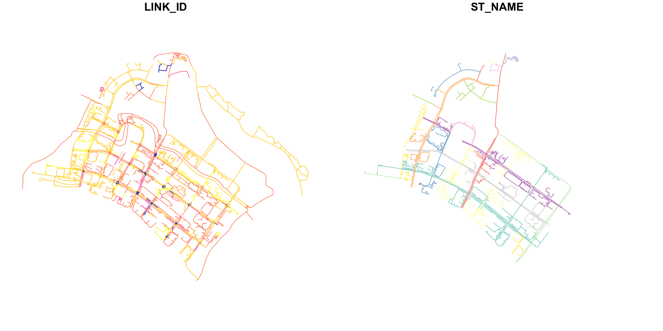
3. plot(st_geometry(network)): Specifically plots only the geometric component of the network object if it is an sf object, which can be useful if you want to focus solely on spatial features. (This is usually what we want.)

plot(st_geometry(network))
plot(childcare,add=T,col='red',pch=19)

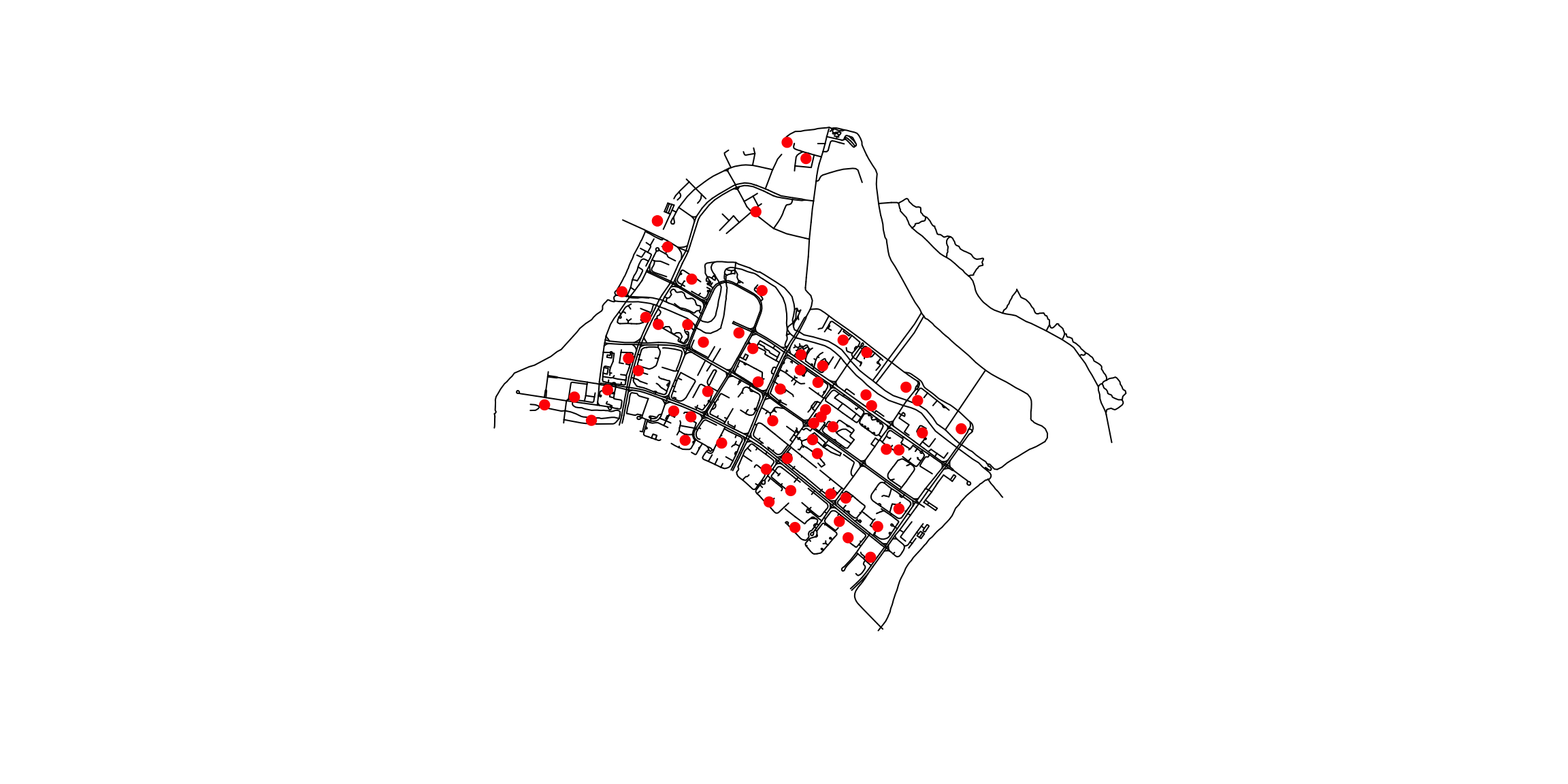
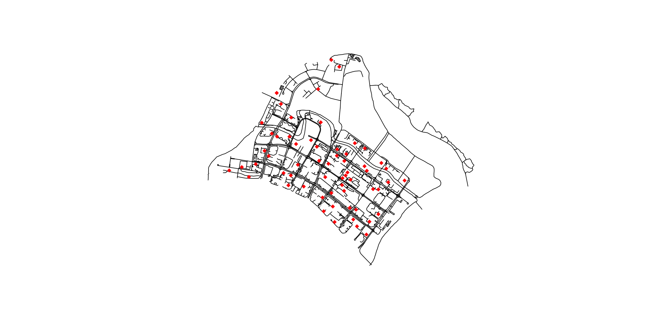
5 Tip 3: Use tmap to create more advanced, complex maps

In Tip 2, we discussed map plotting using plot() from base R. It is fast for quick viz, but lacks customization as compared to libraries such as tmap

Using plot

plot(st_geometry(network))
plot(childcare,add=T,col='red',pch = 18)

Using tmap

We have more mapping options / control and ability to create interactive maps etc.

tmap_mode('view')
tm_shape(childcare) +
  tm_dots(col = 'red') +
  tm_shape(network) +
  tm_lines()

tmap_mode('plot')

6 Tip 4: Preparing Lixel Objects

lixels <- lixelize_lines(network,700,mindist=350)

The choice of 700m is based on NTU research on people’s willingness to walk. The values of lixel length and mindist varies, depending on your research area, eg. walking commuters, cars, etc.

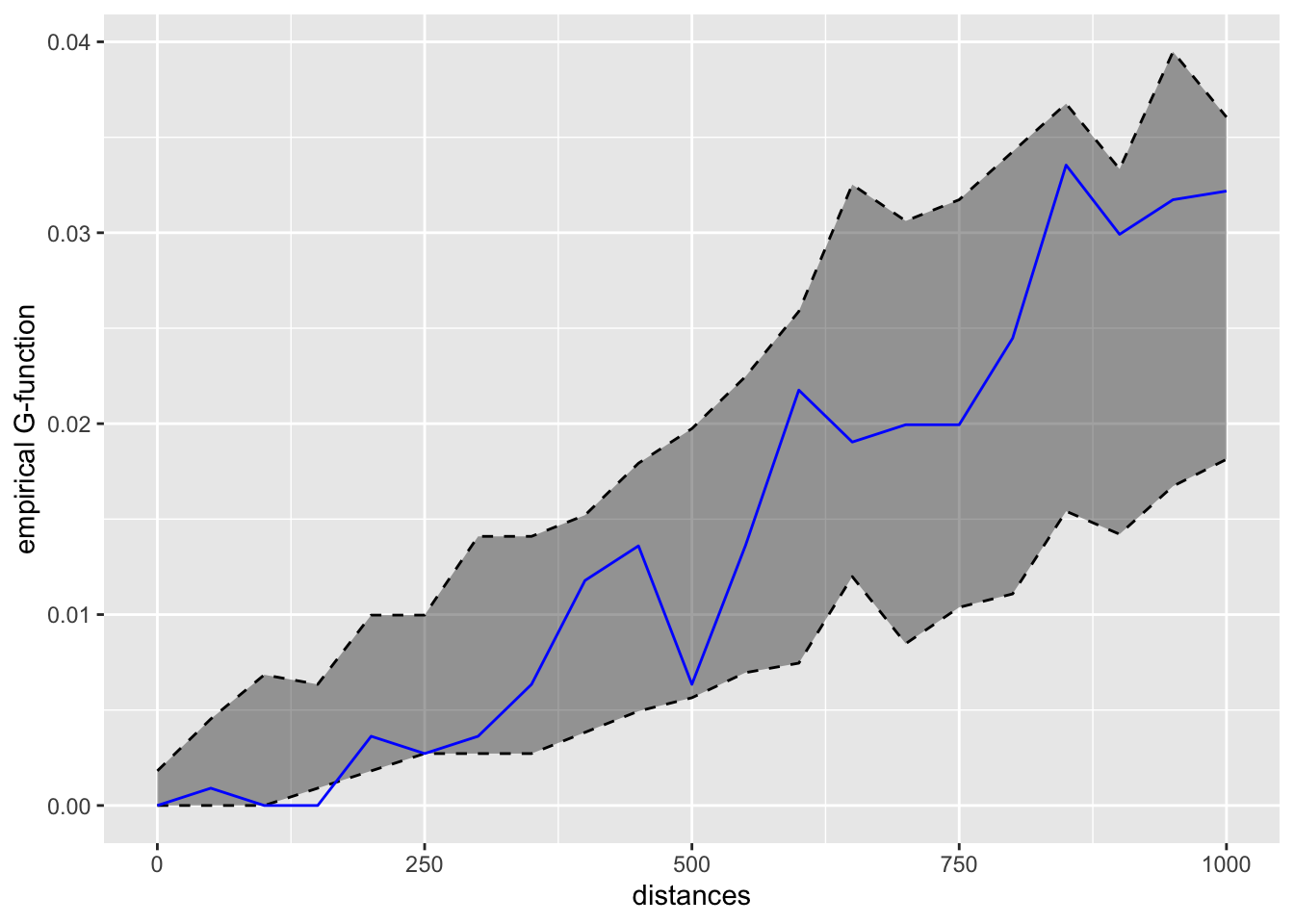
7 Tip 5: Difference between K-Function and G-Function

Reference Link: Network k Functions

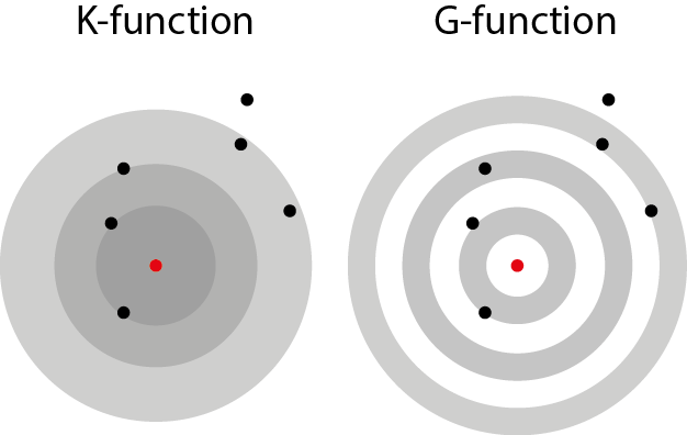
• K-Function (Disc-like): The K-function calculates the proportion of points within a distance r from a typical point. It tells us the “average number of neighbors” around each point within that radius. This measure is cumulative, meaning it looks at all points within growing circles (disks) around a point.

• G-Function (Pair Correlation Function, Ring-like): The G-function is a variation of the K-function that focuses on specific distances rather than cumulative distances. Instead of looking at all points within a growing circle, it examines points within a narrow ring at a specific distance. This allows it to analyze point concentrations at different geographic scales more precisely.

7.1 When to Use K-Function vs. G-Function

• Use the K-Function:
  • When you want to understand the overall pattern of clustering or dispersion of points across various distances.
  • Useful for identifying general trends in the spatial arrangement, such as whether points tend to cluster together or spread out over a broad area.
  • Example: Analyzing the general distribution of trees in a forest to see if they are randomly spaced, clustered, or regularly spaced.
• Use the G-Function:
  • When you are interested in the point concentration at specific distances or scales.
  • Useful for detecting specific scales of clustering or dispersion that might be hidden in the cumulative analysis of the K-function.
  • Example: Studying the distribution of retail stores to understand if there is clustering at a specific distance (e.g., stores tend to cluster within 500 meters of each other but not at larger scales).

kfun_childcare <- kfunctions(network,
                             childcare,
                             start = 0,
                             end = 1000,
                             step = 50,
                             width = 50,
                             nsim = 50,
                             resolution = 50,
                             verbose = FALSE,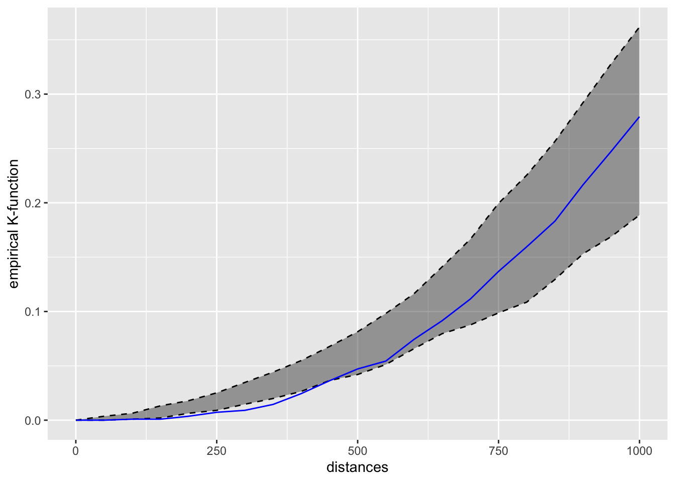
                             conf_int = 0.05)

kfun_childcare$plotk

kfun_childcare$plotg