pacman::p_load(sf, spdep, tmap, tidyverse)5B: Local Measures of Spatial Autocorrelation
In this exercise, we will learn to compute Local Measures of Spatial Autocorrelation (LMSA) using the spdep package, including Local Moran’s I, Getis-Ord’s Gi-statistics, and their visualizations.
1 Exercise 5B Reference
R for Geospatial Data Science and Analytics - 10 Local Measures of Spatial Autocorrelation
2 Overview
Local Measures of Spatial Autocorrelation (LMSA) analyze the relationships between each observation and its surroundings, rather than summarizing these relationships across an entire map. They provide scores that reveal the spatial structure of the data, similar in concept to global measures, and are often mathematically connected, as global measures can be decomposed into local ones.
In this exercise, we will learn to compute Local Measures of Spatial Autocorrelation (LMSA) using the spdep package, including Local Moran’s I, Getis-Ord’s Gi-statistics, and their visualizations.
3 Learning Outcome
- Import geospatial data using the sf package
- Import CSV data using the readr package
- Perform relational joins using the dplyr package
-
Compute
Local Indicator of Spatial Association (LISA) statistics
using spdep
- Detect clusters and outliers with Local Moran’s I
- Identify hot and cold spots with Getis-Ord’s Gi-statistics
- Visualize analysis outputs using the tmap package
4 The Analytical Question
In spatial policy planning, one of the main development objective of the local government and planners is to ensure equal distribution of development in the province. In this study, we will apply spatial statistical methods to examine the distribution of development in Hunan Province, China, using a selected indicator (e.g., GDP per capita).
Our key questions are:
- Is development evenly distributed geographically?
- If not, is there evidence of spatial clustering?
- If clustering exists, where are these clusters located?
5 The Data
The following 2 datasets will be used in this exercise.
| Data Set | Description | Format |
|---|---|---|
| Hunan county boundary layer | Geospatial data set representing the county boundaries of Hunan | ESRI Shapefile |
| Hunan_2012.csv | Contains selected local development indicators for Hunan in 2012 | CSV |
6 Installing and Launching the R Packages
The following R packages will be used in this exercise:
| Package | Purpose | Use Case in Exercise |
|---|---|---|
| sf | Handles spatial data, particularly vector-based geospatial data. | Importing and managing township boundary data for Myanmar. |
| rgdal | Provides bindings to the Geospatial Data Abstraction Library (GDAL) for reading and writing spatial data. | Reading and writing geospatial data in various formats, including shapefiles. |
| spdep | Analyzes spatial dependence and provides tools for spatial econometrics. | Performing spatially constrained clustering and other spatial dependence analyses. |
| tidyverse | A collection of packages for data science tasks like data manipulation and visualization. | Handling attribute data, reading CSV files, and data wrangling with readr, dplyr, and ggplot2. |
| tmap | Creates static and interactive thematic maps. | Visualizing data using choropleth maps to display spatial patterns and relationships. |
| corrplot | Visualizes correlation matrices. | Creating correlation plots to explore relationships between different ICT measures. |
| ggpubr | Provides functions to create and customize ‘ggplot2’-based publication-ready plots. | Enhancing multivariate data visualizations for clearer presentation of results. |
| heatmaply | Generates interactive heatmaps. | Visualizing multivariate data through interactive heatmaps for deeper insights. |
| cluster | Performs cluster analysis. | Conducting hierarchical clustering to group similar regions based on ICT measures. |
| ClustGeo | Performs spatially constrained hierarchical clustering. | Applying spatial constraints to hierarchical clustering for identifying homogeneous regions. |
To install and load these packages, use the following code:
7 Import Data and Preparation
In this section, we will perform 3 necessary steps to prepare the data for analysis.
Note
The data preparation is the same as previous exercise such as Exercise 4A.
7.1 Import Geospatial Shapefile
Firstly, we will use
st_read()
of sf package to import Hunan shapefile into R.
The imported shapefile will be
simple features Object of sf.
hunan <- st_read(dsn = "data/geospatial",
                 layer = "Hunan")
Reading layer `Hunan' from data source
`/Users/walter/code/isss626/isss626-gaa/Hands-on_Ex/Hands-on_Ex05/data/geospatial'
using driver `ESRI Shapefile'
Simple feature collection with 88 features and 7 fields
Geometry type: POLYGON
Dimension: XY
Bounding box: xmin: 108.7831 ymin: 24.6342 xmax: 114.2544 ymax: 30.12812
Geodetic CRS: WGS 847.2 Import Aspatial csv File
Next, we will import Hunan_2012.csv into R by using
read_csv() of readr package. The
output is R dataframe class.
hunan2012 <- read_csv("data/aspatial/Hunan_2012.csv")7.3 Perform Relational Join
Then, we will perform a left_join() to update the
attribute table of hunan’s SpatialPolygonsDataFrame with the
attribute fields of hunan2012 dataframe.
hunan <- left_join(hunan,hunan2012) %>%
  select(1:4, 7, 15)
7.4 Visualizing Regional Development Indicator
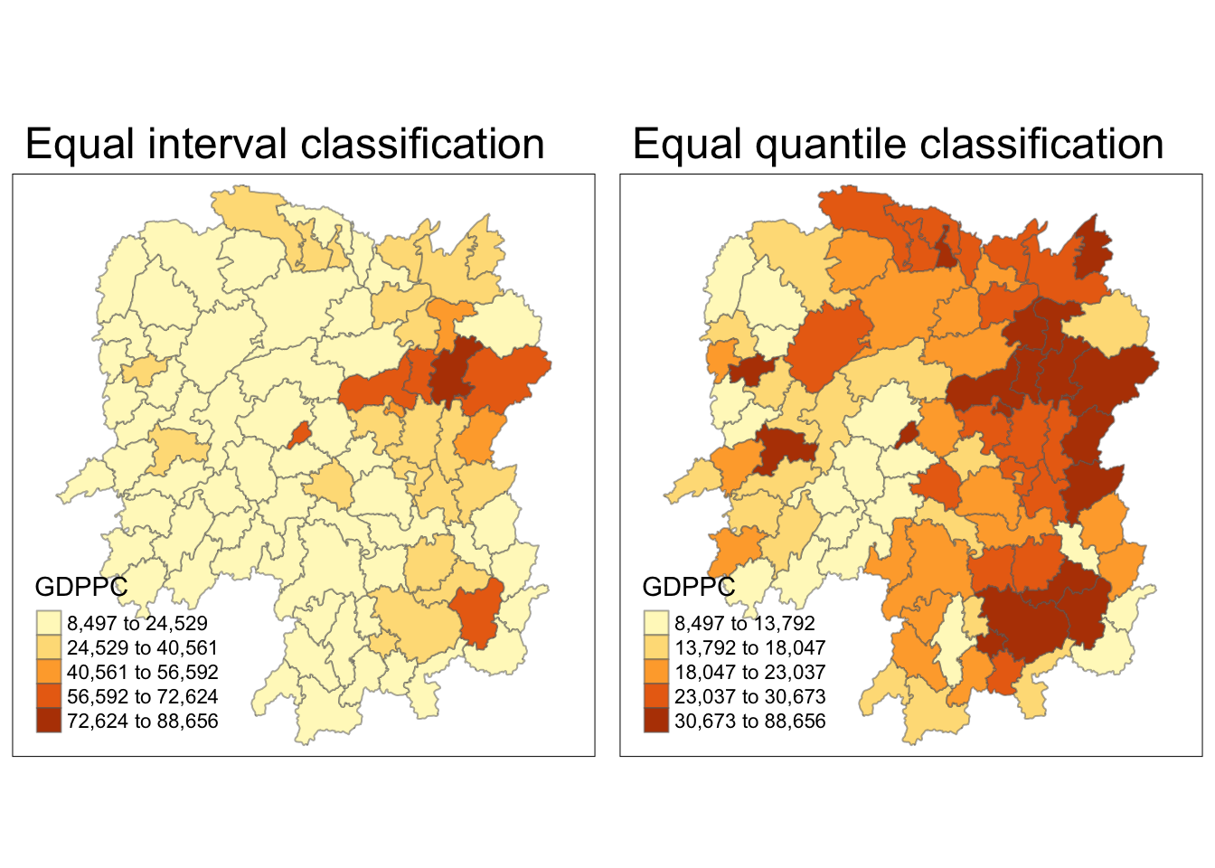
To visualize the regional development indicator, we can prepare a
base map and a choropleth map to show the distribution of GDPPC
2012 (GDP per capita) by using qtm() of
tmap package.
equal <- tm_shape(hunan) +
  tm_fill("GDPPC",
          n = 5,
          style = "equal") +
  tm_borders(alpha = 0.5) +
  tm_layout(main.title = "Equal interval classification")

quantile <- tm_shape(hunan) +
  tm_fill("GDPPC",
          n = 5,
          style = "quantile") +
  tm_borders(alpha = 0.5) +
  tm_layout(main.title = "Equal quantile classification")

tmap_arrange(equal,
             quantile,
             asp=1,
             ncol=2)
8 Local Indicators of Spatial Association(LISA)
Local Indicators of Spatial Association (LISA) are statistics used to identify clusters and outliers in the spatial distribution of a variable. For example, if we are analyzing the GDP per capita in Hunan Province, China, LISA can help detect areas (counties) where GDP values are significantly higher or lower than expected by chance. This means that these values deviate from what would be seen in a random distribution across space.
In this section, we will apply appropriate Local Indicators for Spatial Association (LISA), particularly the Local Moran’s I statistic, to identify clusters and outliers in the 2012 GDP per capita data for Hunan Province.
8.1 Computing Contiguity Spatial Weights
Before we can compute the global spatial autocorrelation statistics, we need to construct a spatial weights of the study area. The spatial weights is used to define the neighbourhood relationships between the geographical units (i.e. county) in the study area.
In the code block below, the poly2nb() function from
the spdep package calculates contiguity weight
matrices for the study area by identifying regions that share
boundaries.
By default, poly2nb() uses the “Queen” criteria,
which considers any shared boundary or corner as a neighbor
(equivalent to setting queen = TRUE). If we want to
restrict the criteria to shared boundaries only (excluding
corners), set queen = FALSE.
wm_q <- poly2nb(hunan,
                queen=TRUE)
summary(wm_q)
Neighbour list object:
Number of regions: 88
Number of nonzero links: 448
Percentage nonzero weights: 5.785124
Average number of links: 5.090909
Link number distribution:
1 2 3 4 5 6 7 8 9 11
2 2 12 16 24 14 11 4 2 1
2 least connected regions:
30 65 with 1 link
1 most connected region:
85 with 11 linksThe summary report above shows that there are 88 area units in Hunan. The most connected area unit has 11 neighbours. There are two area units with only one neighbours.
8.2 Row-standardised Weights Matrix
Next, we need to assign weights to each neighboring polygon. In this case, we’ll use equal weights (style=“W”), where each neighboring polygon gets a weight of 1/(number of neighbors). This means we take the value for each neighbor and divide it by the total number of neighbors, then sum these weighted values to calculate a summary measure, such as weighted income.
While this equal weighting approach is straightforward and easy to understand, it has a limitation: polygons on the edges of the study area have fewer neighbors, which can lead to over- or underestimation of the actual spatial relationships (spatial autocorrelation) in the data.
Tip
For simplicity, we use the style=“W” option in this example, but keep in mind that other, potentially more accurate methods are available, such as style=“B”.
rswm_q <- nb2listw(wm_q, style="W", zero.policy = TRUE)
rswm_q
Characteristics of weights list object:
Neighbour list object:
Number of regions: 88
Number of nonzero links: 448
Percentage nonzero weights: 5.785124
Average number of links: 5.090909
Weights style: W
Weights constants summary:
n nn S0 S1 S2
W 88 7744 88 37.86334 365.9147Tip
-
The input of
nb2listw()must be an object of class nb. The syntax of the function has two major arguments, namely style and zero.poly. -
style can take values “W”, “B”, “C”, “U”, “minmax” and “S”. B is the basic binary coding, W is row standardised (sums over all links to n), C is globally standardised (sums over all links to n), U is equal to C divided by the number of neighbours (sums over all links to unity), while S is the variance-stabilizing coding scheme proposed by Tiefelsdorf et al. 1999, p. 167-168 (sums over all links to n).
-
The zero.policy=TRUE option allows for lists of non-neighbors. This should be used with caution since the user may not be aware of missing neighbors in their dataset however, a zero.policy of FALSE would return an error.
8.3 Computing Local Moran’s I
To compute local Moran’s I, the localmoran() function of spdep will be used. It computes Ii values, given a set of zi values and a listw object providing neighbour weighting information for the polygon associated with the zi values.
First, we compute a vector fips that contains the
indexes to sort the County column of the hunan
dataset in ascending alphabetical order.
fips <- order(hunan$County)
glimpse(hunan$County[fips])
chr [1:88] "Anhua" "Anren" "Anxiang" "Baojing" "Chaling" "Changning" ...Then, we compute local Moran’s I of GDPPC2012 at the county level.
localMI <- localmoran(hunan$GDPPC, rswm_q)

head(localMI)
Ii E.Ii Var.Ii Z.Ii Pr(z != E(Ii))
1 -0.001468468 -2.815006e-05 4.723841e-04 -0.06626904 0.9471636
2 0.025878173 -6.061953e-04 1.016664e-02 0.26266425 0.7928094
3 -0.011987646 -5.366648e-03 1.133362e-01 -0.01966705 0.9843090
4 0.001022468 -2.404783e-07 5.105969e-06 0.45259801 0.6508382
5 0.014814881 -6.829362e-05 1.449949e-03 0.39085814 0.6959021
6 -0.038793829 -3.860263e-04 6.475559e-03 -0.47728835 0.6331568Tip
localmoran() function returns a matrix of values whose columns are:
- Ii: the local Moran’s I statistics
- E.Ii: the expectation of local moran statistic under the randomisation hypothesis
- Var.Ii: the variance of local moran statistic under the randomisation hypothesis
- Z.Ii:the standard deviate of local moran statistic
- Pr(): the p-value of local moran statistic
Next, we list the content of the local Moran matrix derived by using printCoefmat().
printCoefmat(data.frame(
  localMI[fips,],
  row.names=hunan$County[fips]),
  check.names=FALSE)
Ii E.Ii Var.Ii Z.Ii Pr.z....E.Ii..
Anhua -2.2493e-02 -5.0048e-03 5.8235e-02 -7.2467e-02 0.9422
Anren -3.9932e-01 -7.0111e-03 7.0348e-02 -1.4791e+00 0.1391
Anxiang -1.4685e-03 -2.8150e-05 4.7238e-04 -6.6269e-02 0.9472
Baojing 3.4737e-01 -5.0089e-03 8.3636e-02 1.2185e+00 0.2230
Chaling 2.0559e-02 -9.6812e-04 2.7711e-02 1.2932e-01 0.8971
Changning -2.9868e-05 -9.0010e-09 1.5105e-07 -7.6828e-02 0.9388
Changsha 4.9022e+00 -2.1348e-01 2.3194e+00 3.3590e+00 0.0008
Chengbu 7.3725e-01 -1.0534e-02 2.2132e-01 1.5895e+00 0.1119
Chenxi 1.4544e-01 -2.8156e-03 4.7116e-02 6.8299e-01 0.4946
Cili 7.3176e-02 -1.6747e-03 4.7902e-02 3.4200e-01 0.7324
Dao 2.1420e-01 -2.0824e-03 4.4123e-02 1.0297e+00 0.3032
Dongan 1.5210e-01 -6.3485e-04 1.3471e-02 1.3159e+00 0.1882
Dongkou 5.2918e-01 -6.4461e-03 1.0748e-01 1.6338e+00 0.1023
Fenghuang 1.8013e-01 -6.2832e-03 1.3257e-01 5.1198e-01 0.6087
Guidong -5.9160e-01 -1.3086e-02 3.7003e-01 -9.5104e-01 0.3416
Guiyang 1.8240e-01 -3.6908e-03 3.2610e-02 1.0305e+00 0.3028
Guzhang 2.8466e-01 -8.5054e-03 1.4152e-01 7.7931e-01 0.4358
Hanshou 2.5878e-02 -6.0620e-04 1.0167e-02 2.6266e-01 0.7928
Hengdong 9.9964e-03 -4.9063e-04 6.7742e-03 1.2742e-01 0.8986
Hengnan 2.8064e-02 -3.2160e-04 3.7597e-03 4.6294e-01 0.6434
Hengshan -5.8201e-03 -3.0437e-05 5.1076e-04 -2.5618e-01 0.7978
Hengyang 6.2997e-02 -1.3046e-03 2.1865e-02 4.3486e-01 0.6637
Hongjiang 1.8790e-01 -2.3019e-03 3.1725e-02 1.0678e+00 0.2856
Huarong -1.5389e-02 -1.8667e-03 8.1030e-02 -4.7503e-02 0.9621
Huayuan 8.3772e-02 -8.5569e-04 2.4495e-02 5.4072e-01 0.5887
Huitong 2.5997e-01 -5.2447e-03 1.1077e-01 7.9685e-01 0.4255
Jiahe -1.2431e-01 -3.0550e-03 5.1111e-02 -5.3633e-01 0.5917
Jianghua 2.8651e-01 -3.8280e-03 8.0968e-02 1.0204e+00 0.3076
Jiangyong 2.4337e-01 -2.7082e-03 1.1746e-01 7.1800e-01 0.4728
Jingzhou 1.8270e-01 -8.5106e-04 2.4363e-02 1.1759e+00 0.2396
Jinshi -1.1988e-02 -5.3666e-03 1.1334e-01 -1.9667e-02 0.9843
Jishou -2.8680e-01 -2.6305e-03 4.4028e-02 -1.3543e+00 0.1756
Lanshan 6.3334e-02 -9.6365e-04 2.0441e-02 4.4972e-01 0.6529
Leiyang 1.1581e-02 -1.4948e-04 2.5082e-03 2.3422e-01 0.8148
Lengshuijiang -1.7903e+00 -8.2129e-02 2.1598e+00 -1.1623e+00 0.2451
Li 1.0225e-03 -2.4048e-07 5.1060e-06 4.5260e-01 0.6508
Lianyuan -1.4672e-01 -1.8983e-03 1.9145e-02 -1.0467e+00 0.2952
Liling 1.3774e+00 -1.5097e-02 4.2601e-01 2.1335e+00 0.0329
Linli 1.4815e-02 -6.8294e-05 1.4499e-03 3.9086e-01 0.6959
Linwu -2.4621e-03 -9.0703e-06 1.9258e-04 -1.7676e-01 0.8597
Linxiang 6.5904e-02 -2.9028e-03 2.5470e-01 1.3634e-01 0.8916
Liuyang 3.3688e+00 -7.7502e-02 1.5180e+00 2.7972e+00 0.0052
Longhui 8.0801e-01 -1.1377e-02 1.5538e-01 2.0787e+00 0.0376
Longshan 7.5663e-01 -1.1100e-02 3.1449e-01 1.3690e+00 0.1710
Luxi 1.8177e-01 -2.4855e-03 3.4249e-02 9.9561e-01 0.3194
Mayang 2.1852e-01 -5.8773e-03 9.8049e-02 7.1663e-01 0.4736
Miluo 1.8704e+00 -1.6927e-02 2.7925e-01 3.5715e+00 0.0004
Nan -9.5789e-03 -4.9497e-04 6.8341e-03 -1.0988e-01 0.9125
Ningxiang 1.5607e+00 -7.3878e-02 8.0012e-01 1.8274e+00 0.0676
Ningyuan 2.0910e-01 -7.0884e-03 8.2306e-02 7.5356e-01 0.4511
Pingjiang -9.8964e-01 -2.6457e-03 5.6027e-02 -4.1698e+00 0.0000
Qidong 1.1806e-01 -2.1207e-03 2.4747e-02 7.6396e-01 0.4449
Qiyang 6.1966e-02 -7.3374e-04 8.5743e-03 6.7712e-01 0.4983
Rucheng -3.6992e-01 -8.8999e-03 2.5272e-01 -7.1814e-01 0.4727
Sangzhi 2.5053e-01 -4.9470e-03 6.8000e-02 9.7972e-01 0.3272
Shaodong -3.2659e-02 -3.6592e-05 5.0546e-04 -1.4510e+00 0.1468
Shaoshan 2.1223e+00 -5.0227e-02 1.3668e+00 1.8583e+00 0.0631
Shaoyang 5.9499e-01 -1.1253e-02 1.3012e-01 1.6807e+00 0.0928
Shimen -3.8794e-02 -3.8603e-04 6.4756e-03 -4.7729e-01 0.6332
Shuangfeng 9.2835e-03 -2.2867e-03 3.1516e-02 6.5174e-02 0.9480
Shuangpai 8.0591e-02 -3.1366e-04 8.9838e-03 8.5358e-01 0.3933
Suining 3.7585e-01 -3.5933e-03 4.1870e-02 1.8544e+00 0.0637
Taojiang -2.5394e-01 -1.2395e-03 1.4477e-02 -2.1002e+00 0.0357
Taoyuan 1.4729e-02 -1.2039e-04 8.5103e-04 5.0903e-01 0.6107
Tongdao 4.6482e-01 -6.9870e-03 1.9879e-01 1.0582e+00 0.2900
Wangcheng 4.4220e+00 -1.1067e-01 1.3596e+00 3.8873e+00 0.0001
Wugang 7.1003e-01 -7.8144e-03 1.0710e-01 2.1935e+00 0.0283
Xiangtan 2.4530e-01 -3.6457e-04 3.2319e-03 4.3213e+00 0.0000
Xiangxiang 2.6271e-01 -1.2703e-03 2.1290e-02 1.8092e+00 0.0704
Xiangyin 5.4525e-01 -4.7442e-03 7.9236e-02 1.9539e+00 0.0507
Xinhua 1.1810e-01 -6.2649e-03 8.6001e-02 4.2409e-01 0.6715
Xinhuang 1.5725e-01 -4.1820e-03 3.6648e-01 2.6667e-01 0.7897
Xinning 6.8928e-01 -9.6674e-03 2.0328e-01 1.5502e+00 0.1211
Xinshao 5.7578e-02 -8.5932e-03 1.1769e-01 1.9289e-01 0.8470
Xintian -7.4050e-03 -5.1493e-03 1.0877e-01 -6.8395e-03 0.9945
Xupu 3.2406e-01 -5.7468e-03 5.7735e-02 1.3726e+00 0.1699
Yanling -6.9021e-02 -5.9211e-04 9.9306e-03 -6.8667e-01 0.4923
Yizhang -2.6844e-01 -2.2463e-03 4.7588e-02 -1.2202e+00 0.2224
Yongshun 6.3064e-01 -1.1350e-02 1.8830e-01 1.4795e+00 0.1390
Yongxing 4.3411e-01 -9.0735e-03 1.5088e-01 1.1409e+00 0.2539
You 7.8750e-02 -7.2728e-03 1.2116e-01 2.4714e-01 0.8048
Yuanjiang 2.0004e-04 -1.7760e-04 2.9798e-03 6.9181e-03 0.9945
Yuanling 8.7298e-03 -2.2981e-06 2.3221e-05 1.8121e+00 0.0700
Yueyang 4.1189e-02 -1.9768e-04 2.3113e-03 8.6085e-01 0.3893
Zhijiang 1.0476e-01 -7.8123e-04 1.3100e-02 9.2214e-01 0.3565
Zhongfang -2.2685e-01 -2.1455e-03 3.5927e-02 -1.1855e+00 0.2358
Zhuzhou 3.2864e-01 -5.2432e-04 7.2391e-03 3.8688e+00 0.0001
Zixing -7.6849e-01 -8.8210e-02 9.4057e-01 -7.0144e-01 0.48308.3.1 Mapping the Local Moran’s I
Before mapping the local Moran’s I map, we append the local
Moran’s I dataframe (i.e. localMI) onto hunan
SpatialPolygonDataFrame, hunan.localMI.
Simple feature collection with 6 features and 11 fields
Geometry type: POLYGON
Dimension:     XY
Bounding box:  xmin: 110.4922 ymin: 28.61762 xmax: 112.3013 ymax: 30.12812
Geodetic CRS:  WGS 84
   NAME_2  ID_3  NAME_3   ENGTYPE_3  County GDPPC           Ii          E.Ii
1 Changde 21098 Anxiang      County Anxiang 23667 -0.001468468 -2.815006e-05
2 Changde 21100 Hanshou      County Hanshou 20981  0.025878173 -6.061953e-04
3 Changde 21101  Jinshi County City  Jinshi 34592 -0.011987646 -5.366648e-03
4 Changde 21102      Li      County      Li 24473  0.001022468 -2.404783e-07
5 Changde 21103   Linli      County   Linli 25554  0.014814881 -6.829362e-05
6 Changde 21104  Shimen      County  Shimen 27137 -0.038793829 -3.860263e-04
        Var.Ii        Z.Ii     Pr.Ii                       geometry
1 4.723841e-04 -0.06626904 0.9471636 POLYGON ((112.0625 29.75523...
2 1.016664e-02  0.26266425 0.7928094 POLYGON ((112.2288 29.11684...
3 1.133362e-01 -0.01966705 0.9843090 POLYGON ((111.8927 29.6013,...
4 5.105969e-06  0.45259801 0.6508382 POLYGON ((111.3731 29.94649...
5 1.449949e-03  0.39085814 0.6959021 POLYGON ((111.6324 29.76288...
6 6.475559e-03 -0.47728835 0.6331568 POLYGON ((110.8825 30.11675...
8.3.2 Mapping local Moran’s I values
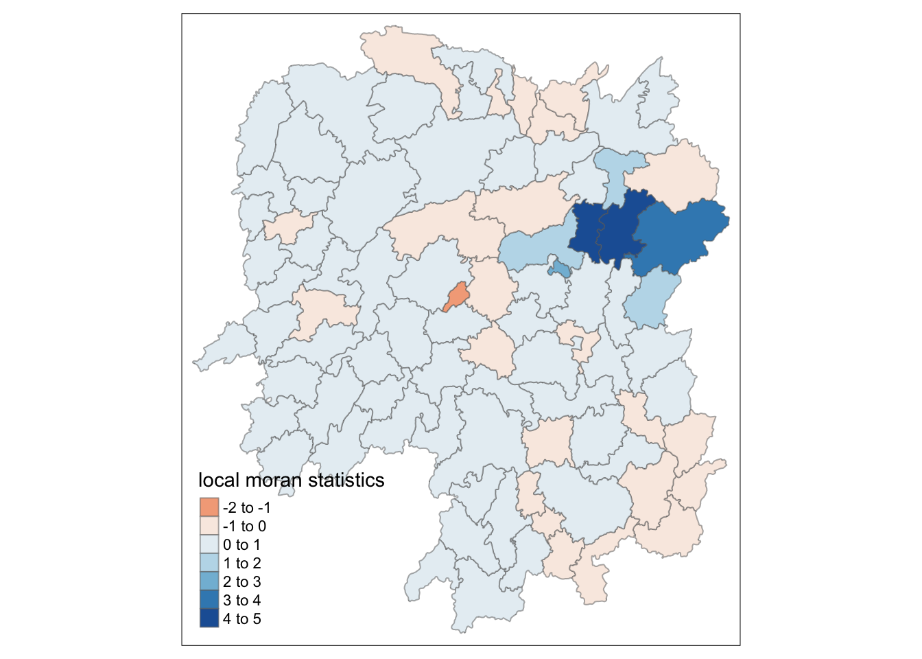
We can plot the local Moran’s I values using choropleth mapping functions of tmap package.
tm_shape(hunan.localMI) +
  tm_fill(col = "Ii",
          style = "pretty",
          palette = "RdBu",
          title = "local moran statistics") +
  tm_borders(alpha = 0.5)
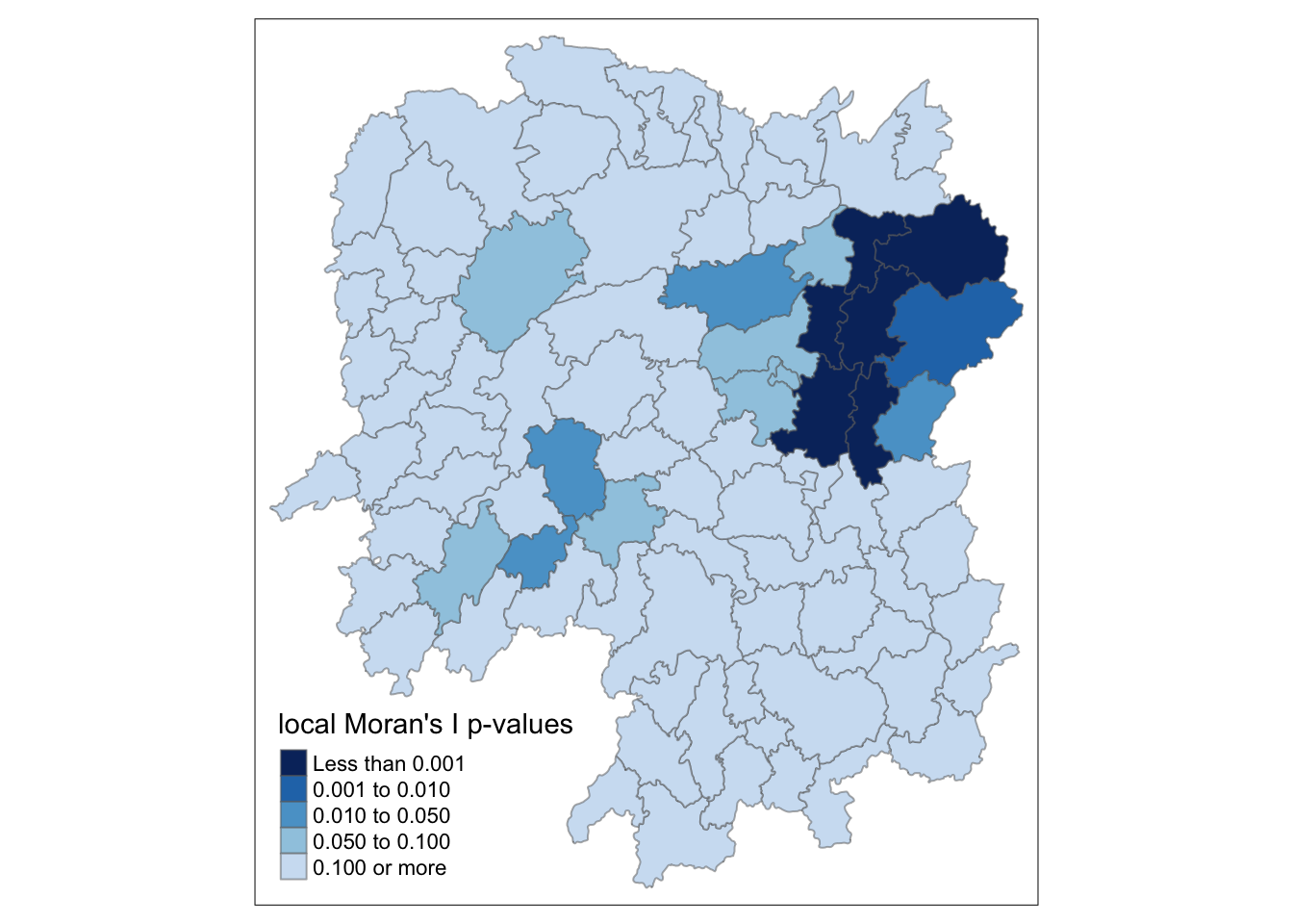
8.3.3 Mapping local Moran’s I p-values
The choropleth shows there is evidence for both positive and negative Ii values. However, it is useful to consider the p-values for each of these values
The code block below produce a choropleth map of Moran’s I p-values by using functions of tmap package.
tm_shape(hunan.localMI) +
  tm_fill(col = "Pr.Ii",
          breaks=c(-Inf, 0.001, 0.01, 0.05, 0.1, Inf),
          palette="-Blues",
          title = "local Moran's I p-values") +
  tm_borders(alpha = 0.5)
8.3.4 Mapping both local Moran’s I values and p-values
For effective interpretation, it is better to plot both the local Moran’s I values map and its corresponding p-values map next to each other.
The code block below will be used to create such visualisation.
localMI.map <- tm_shape(hunan.localMI) +
  tm_fill(col = "Ii",
          style = "pretty",
          title = "local moran statistics") +
  tm_borders(alpha = 0.5)

pvalue.map <- tm_shape(hunan.localMI) +
  tm_fill(col = "Pr.Ii",
          breaks=c(-Inf, 0.001, 0.01, 0.05, 0.1, Inf),
          palette="-Blues",
          title = "local Moran's I p-values") +
  tm_borders(alpha = 0.5)

tmap_arrange(localMI.map, pvalue.map, asp=1, ncol=2)

# find county with max Ii and observe its Ii, p-value
max_row <- hunan.localMI[which.max(hunan.localMI$Ii), , drop = FALSE]
max_row
Simple feature collection with 1 feature and 11 fields
Geometry type: POLYGON
Dimension: XY
Bounding box: xmin: 112.8907 ymin: 27.91915 xmax: 113.506 ymax: 28.66025
Geodetic CRS: WGS 84
NAME_2 ID_3 NAME_3 ENGTYPE_3 County GDPPC Ii E.Ii
84 Changsha 21107 Changsha District Changsha 88656 4.902202 -0.2134796
Var.Ii Z.Ii Pr.Ii geometry
84 2.319447 3.35901 0.0007822232 POLYGON ((112.9421 28.03722...# find county with max Ii and observe its Ii, p-value
min_row <- hunan.localMI[which.min(hunan.localMI$Ii), , drop = FALSE]
min_rowSimple feature collection with 1 feature and 11 fields
Geometry type: POLYGON
Dimension: XY
Bounding box: xmin: 111.3138 ymin: 27.53506 xmax: 111.6069 ymax: 27.81732
Geodetic CRS: WGS 84
NAME_2 ID_3 NAME_3 ENGTYPE_3 County GDPPC Ii
34 Loudi 21143 Lengshuijiang County City Lengshuijiang 64257 -1.790335
E.Ii Var.Ii Z.Ii Pr.Ii geometry
34 -0.08212937 2.159843 -1.162329 0.245102 POLYGON ((111.5307 27.81472...Note
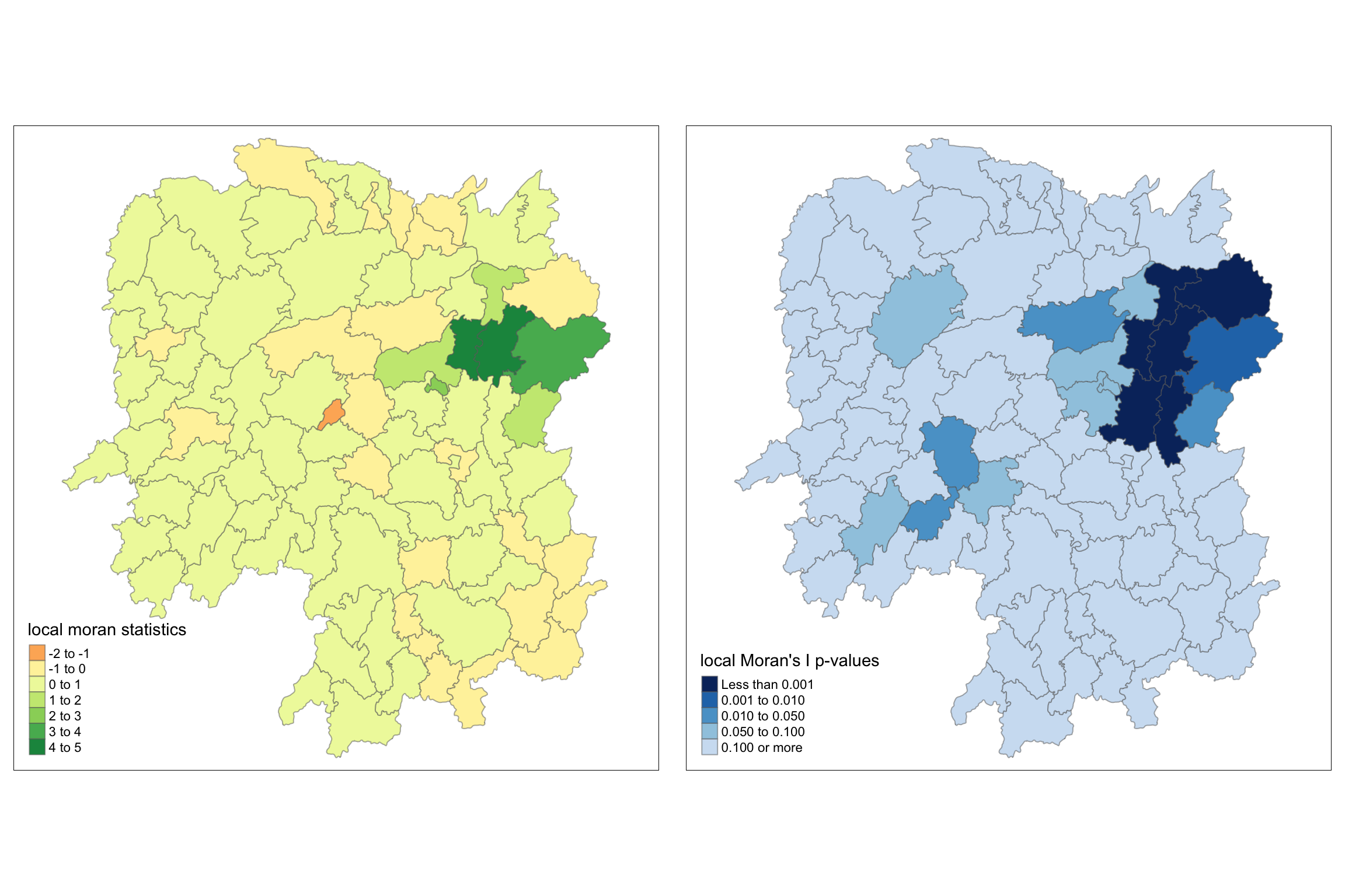
The plot above consists of two maps: one showing the Local
Moran’s I statistics (Ii) and the other
displaying the corresponding p-values for Local Moran’s I
statistics.
8.3.4.1 Left Plot: Local Moran’s I Statistics
Color Scale: - The color scale ranges
from light yellow to dark green, representing different
ranges of Local Moran’s I values (Ii).
-
Dark Green Areas: Represent counties with high positive Local Moran’s I values (between 3 and 5). These areas show strong positive spatial autocorrelation, indicating clusters where counties have similar high GDP per capita values compared to their neighbors.
-
Light Yellow Areas: Represent counties with lower Local Moran’s I values (around 0 to 1). These areas have weaker spatial autocorrelation, suggesting less significant clustering or similarity with their neighbors.
-
Orange Areas: Represent negative Local Moran’s I values (between -2 to 0). These are areas where counties have significantly different GDP per capita values from their neighbors (spatial outliers).
8.3.4.2 Right Plot: Local Moran’s I p-values
Color Scale: - The color scale ranges from light blue to dark blue, representing different ranges of p-values for Local Moran’s I statistics.
-
Dark Blue Areas: Represent counties with very low p-values (less than 0.001), indicating that the observed spatial clustering is statistically significant at a very high confidence level.
-
Lighter Blue Areas: Represent counties with higher p-values (e.g., between 0.01 and 0.10), suggesting that the clustering is less statistically significant.
-
Very Light Blue Areas: Represent counties with p-values greater than 0.10, indicating that there is no statistically significant spatial autocorrelation.
8.3.4.3 Observations:
- The map shows that the central-eastern region (around the Changsha county) has several dark blue counties with very low p-values, indicating strong evidence of significant spatial clustering of similar GDP per capita values.
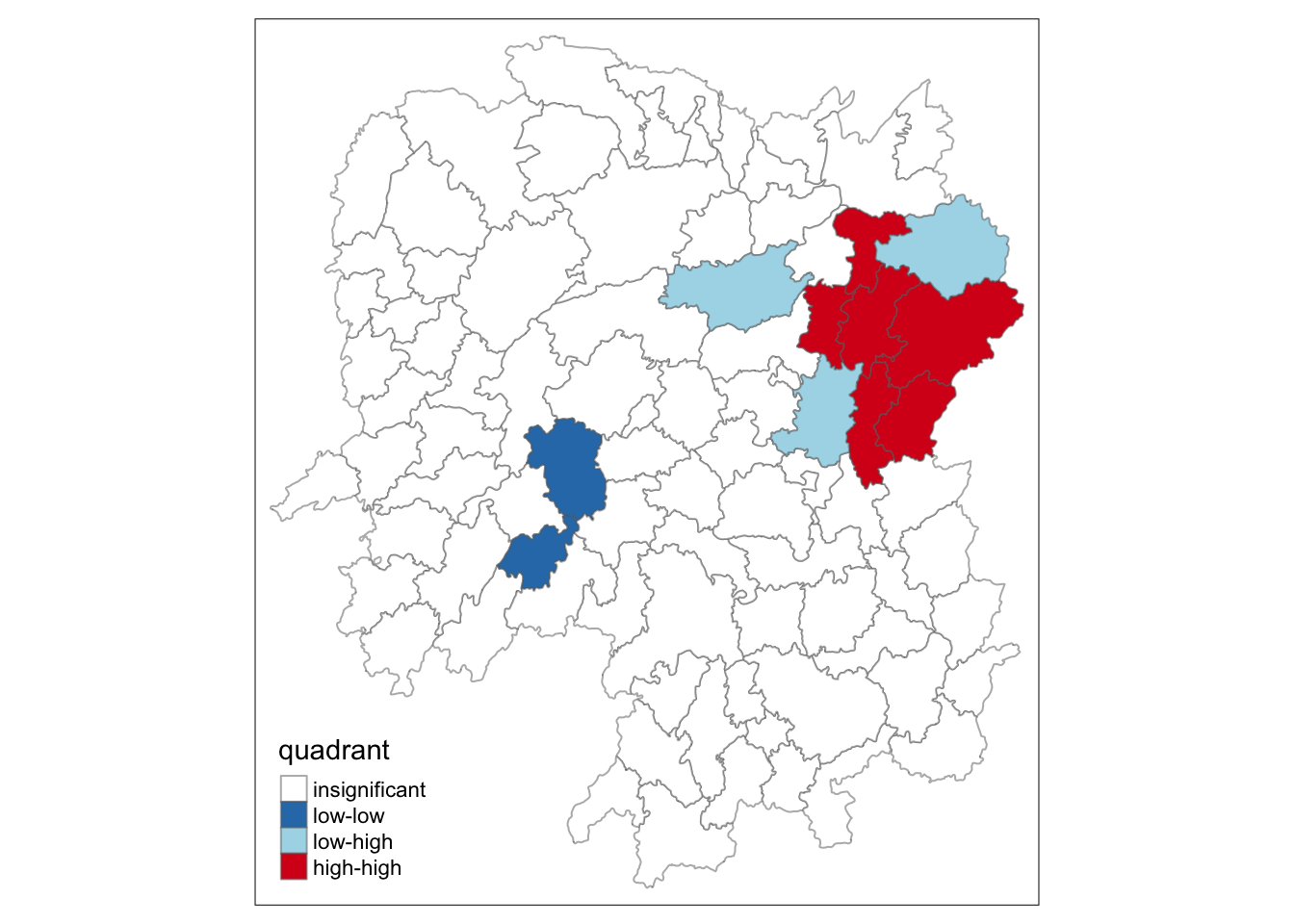
9 Creating a LISA Cluster Map
The LISA Cluster Map shows the significant locations color coded by type of spatial autocorrelation.
Before we can generate the LISA cluster map, we have to plot the Moran scatterplot.
9.1 Plotting Moran scatterplot
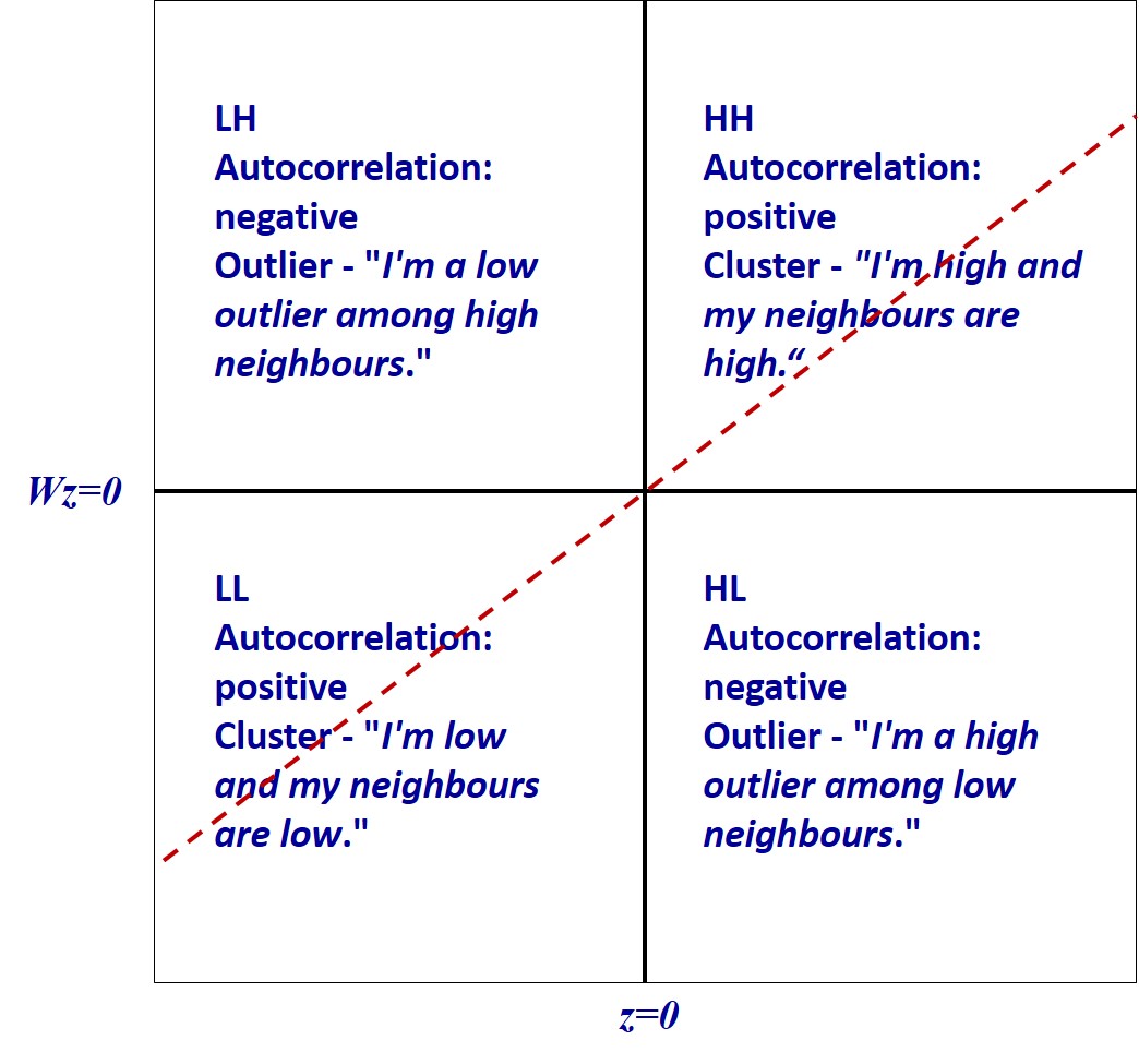
The Moran scatterplot is an illustration of the relationship between the values of the chosen attribute at each location and the average value of the same attribute at neighboring locations.
The code block below plots the Moran scatterplot of GDPPC 2012 by using moran.plot() of spdep.
nci <- moran.plot(hunan$GDPPC, rswm_q,
                  labels=as.character(hunan$County),
                  xlab="GDPPC 2012",
                  ylab="Spatially Lag GDPPC 2012")
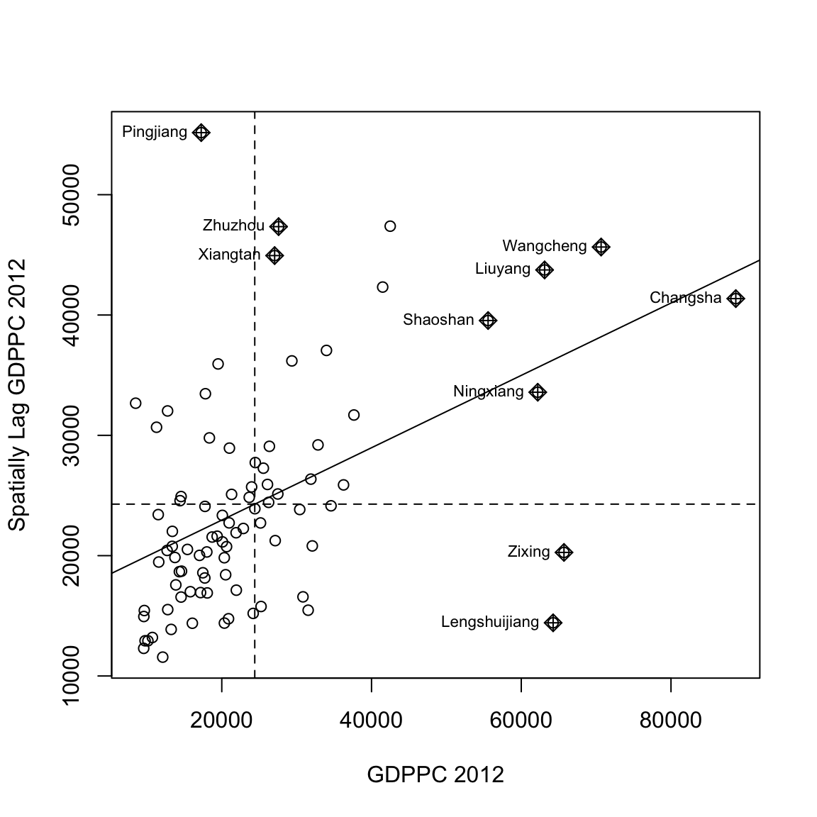
Note
Observations The plot is split in 4 quadrants. The top right corner belongs to areas that have high GDPPC and are surrounded by other areas that have the average level of GDPPC. This are the high-high locations in the lesson slide, recall:
9.2 Plotting Moran scatterplot with Standardised Variable
To plot Moran scatterplot with standardised variable:
-
Use
scale()to center and scale the variable. Centering is done by subtracting the mean (omitting NAs) the corresponding columns, and scaling is done by dividing the (centered) variable by their standard deviations. -
Use
as.vector()to ensure that the standardized output is treated as a vector, which is necessary for proper mapping into the output data frame. Plot the Moran scatterplot
hunan$Z.GDPPC <- scale(hunan$GDPPC) %>%
  as.vector
nci2 <- moran.plot(hunan$Z.GDPPC, rswm_q,
labels=as.character(hunan$County),
xlab="z-GDPPC 2012",
ylab="Spatially Lag z-GDPPC 2012")
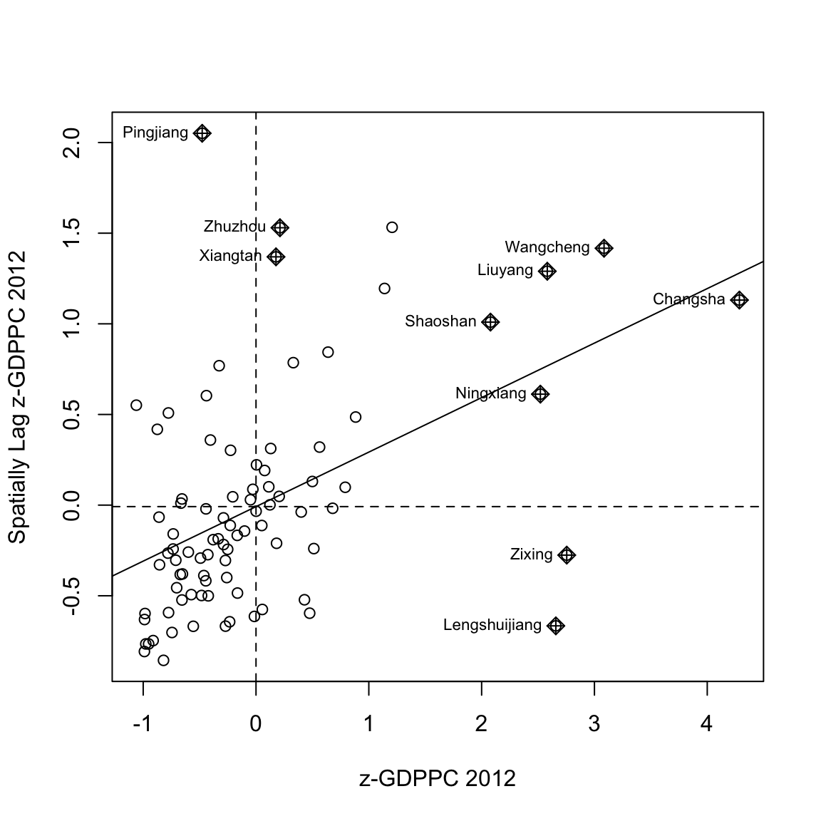
Note
Note that the plot is similar to the previous plot. After scaling it, the cut off axis for x and y-axis is at 0.
9.3 Preparing LISA map classes
The code block below show the steps to prepare a LISA cluster map.
- Convert to Vector
- derive the spatially lagged variable of interest (i.e. GDPPC) and centers the spatially lagged variable around its mean.
hunan$lag_GDPPC <- lag.listw(rswm_q,
                             hunan$GDPPC)

DV <- hunan$lag_GDPPC - mean(hunan$lag_GDPPC) - center the local Moran’s variable around the mean.
LM_I <- localMI[,1] - mean(localMI[,1]) - set a statistical significance level (alpha value) for the local Moran.
signif <- 0.05 - define quadrants. The four command lines define the low-low (1), low-high (2), high-low (3) and high-high (4) categories.
quadrant[DV <0 & LM_I>0] <- 1
quadrant[DV >0 & LM_I<0] <- 2
quadrant[DV <0 & LM_I<0] <- 3
quadrant[DV >0 & LM_I>0] <- 4 - place non-significant Moran in the category 0.
quadrant[localMI[,5]>signif] <- 09.4 Plotting LISA map
Now, we can build the LISA map:
hunan.localMI$quadrant <- quadrant
colors <- c("#ffffff", "#2c7bb6", "#abd9e9", "#fdae61", "#d7191c")
clusters <- c("insignificant", "low-low", "low-high", "high-low", "high-high")

tm_shape(hunan.localMI) +
  tm_fill(col = "quadrant",
          style = "cat",
          palette = colors[c(sort(unique(quadrant)))+1],
          labels = clusters[c(sort(unique(quadrant)))+1],
          popup.vars = c("")) +
  tm_view(set.zoom.limits = c(11,17)) +
  tm_borders(alpha=0.5)
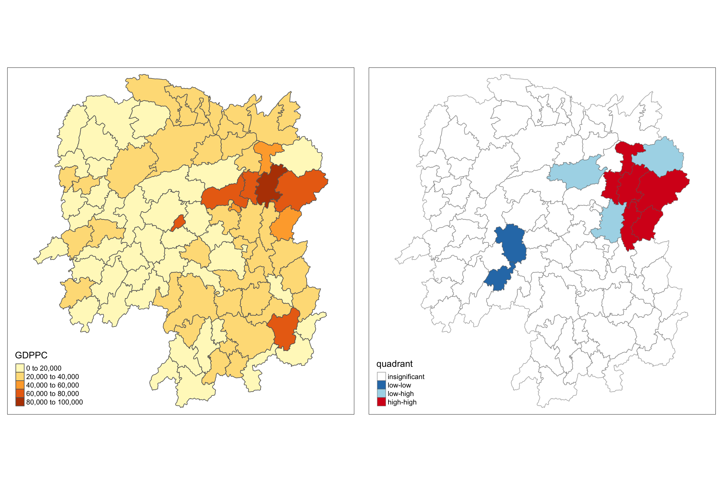
For effective interpretation, it is better to plot both the local Moran’s I values map and its corresponding p-values map next to each other.
To create such visualisation:
gdppc <- qtm(hunan, "GDPPC")

hunan.localMI$quadrant <- quadrant
colors <- c("#ffffff", "#2c7bb6", "#abd9e9", "#fdae61", "#d7191c")
clusters <- c("insignificant", "low-low", "low-high", "high-low", "high-high")

LISAmap <- tm_shape(hunan.localMI) +
  tm_fill(col = "quadrant",
          style = "cat",
          palette = colors[c(sort(unique(quadrant)))+1],
          labels = clusters[c(sort(unique(quadrant)))+1],
          popup.vars = c("")) +
  tm_view(set.zoom.limits = c(11,17)) +
  tm_borders(alpha=0.5)

tmap_arrange(gdppc, LISAmap,
             asp=1, ncol=2)
We can also include the local Moran’s I map and p-value map as shown below for easy comparison.
Note
Question: What statistical observations can you draw from the LISA map above?
From the LISA map and GDPPC map, there is a significant “high-high” cluster in the central-eastern part of the province, where counties with high GDP per capita are surrounded by similar counties.
This pattern is reinforced by the Local Moran’s I statistics map, which show the same region in a deep green shade, indicating strong positive spatial autocorrelation. The corresponding low p-values further confirm the statistical significance of this economic clustering.
Notably, the high-high cluster on the LISA map extends over more counties than those highlighted by the Local Moran’s I statistics.
10 Hot Spot and Cold Spot Area Analysis
Beside detecting cluster and outliers, localised spatial statistics can be also used to detect hot spot and/or cold spot areas.
The term ‘hot spot’ has been used generically across disciplines to describe a region or value that is higher relative to its surroundings (Lepers et al 2005, Aben et al 2012, Isobe et al 2015).
10.1 Getis and Ord’s G-Statistics
An alternative spatial statistics to detect spatial anomalies is the Getis and Ord’s G-statistics (Getis and Ord, 1972; Ord and Getis, 1995). It looks at neighbours within a defined proximity to identify where either high or low values clutser spatially. Here, statistically significant hot-spots are recognised as areas of high values where other areas within a neighbourhood range also share high values too.
The analysis consists of three steps:
- Deriving spatial weight matrix
- Computing Gi statistics
- Mapping Gi statistics
10.2 Deriving Distance-based Weight Matrix
First, we need to define a new set of neighbors. Unlike spatial autocorrelation, which considers units sharing borders, the Getis-Ord method defines neighbors based on distance.
There are two types of distance-based proximity matrices:
- Fixed Distance Weight Matrix: Neighbors are defined within a fixed distance.
- Adaptive Distance Weight Matrix: Neighbors are defined based on a varying distance that adapts to include a specified number of nearest neighbors.
10.2.1 Deriving the Centroid
To create a connectivity graph, we first need to associate
points (centroids) with each polygon in our spatial data. This
process involves more than simply running
st_centroid() on the us.bound sf
object; we need to extract coordinates into a separate data
frame.
We achieve this using a mapping function, which applies a
specific function to each element of a vector and returns a new
vector of the same length. Here, the input vector is the
geometry column of us.bound, and the function
applied is st_centroid(). We’ll use the
map_dbl function from the
purrr package to do this. For more details,
refer to the
map documentation.
To extract longitude values, we map the
st_centroid() function over the geometry column of
us.bound and access the longitude using double
bracket notation [[ ]] and 1, which
retrieves the first value (longitude) from each centroid.
longitude <- map_dbl(hunan$geometry, ~st_centroid(.x)[[1]])We do the same for latitude with one key difference. We access the second value per each centroid with [[2]].
latitude <- map_dbl(hunan$geometry, ~st_centroid(.x)[[2]])
Now that we have latitude and longitude, we use
cbind to put longitude and latitude into the same
object.
coords <- cbind(longitude, latitude)10.2.2 Determine the Cut-off Distance
To determine the upper limit for the distance band:
-
Use the
knearneigh()function from spdep to create a matrix containing the indices of the k nearest neighbors for each point. -
Convert the
knnobject fromknearneigh()into a neighbor list (nbclass) usingknn2nb(). This list contains integer vectors representing the neighbor region numbers. -
Use
nbdists()from spdep to calculate the lengths of the neighbor relationships (distances). If coordinates are projected, the distances are in the units of the coordinates; otherwise, they are in kilometers. -
Flatten the list structure of the returned distances using
unlist().
#coords <- coordinates(hunan)
k1 <- knn2nb(knearneigh(coords))
k1dists <- unlist(nbdists(k1, coords, longlat = TRUE))
summary(k1dists)
Min. 1st Qu. Median Mean 3rd Qu. Max.
24.79 32.57 38.01 39.07 44.52 61.79 Note
Using the summary report, we can observe that the largest first nearest neighbour distance is 61.79 km, so using this as the upper threshold gives certainty that all units will have at least one neighbour.
10.2.3 Computing Fixed Distance Weight Matrix
Use dnearneigh() to compute distance weight matrix:
# get max dist from k1dists rounded up to integer
max_dist <- as.integer(ceiling(max(k1dists)))

wm_d62 <- dnearneigh(x=coords, d1=0, d2=max_dist, longlat = TRUE)
wm_d62
Neighbour list object:
Number of regions: 88
Number of nonzero links: 324
Percentage nonzero weights: 4.183884
Average number of links: 3.681818 Next, nb2listw() is used to convert the nb object into spatial weights object.
wm62_lw <- nb2listw(wm_d62, style = 'B')
summary(wm62_lw)Characteristics of weights list object:
Neighbour list object:
Number of regions: 88
Number of nonzero links: 324
Percentage nonzero weights: 4.183884
Average number of links: 3.681818
Link number distribution:
1 2 3 4 5 6
6 15 14 26 20 7
6 least connected regions:
6 15 30 32 56 65 with 1 link
7 most connected regions:
21 28 35 45 50 52 82 with 6 links
Weights style: B
Weights constants summary:
n nn S0 S1 S2
B 88 7744 324 648 5440
The output spatial weights object is called
wm62_lw.
10.3 Computing adaptive distance weight matrix
One of the characteristics of fixed distance weight matrix is that more densely settled areas (usually the urban areas) tend to have more neighbours and the less densely settled areas (usually the rural counties) tend to have lesser neighbours. Having many neighbours smoothes the neighbour relationship across more neighbours.
It is possible to control the numbers of neighbours directly using k-nearest neighbours, either accepting asymmetric neighbours or imposing symmetry as shown in the code block below.
# set nearest neighbour as 8
knn <- knn2nb(knearneigh(coords, k=8))
knn
Neighbour list object:
Number of regions: 88
Number of nonzero links: 704
Percentage nonzero weights: 9.090909
Average number of links: 8
Non-symmetric neighbours listNext, nb2listw() is used to convert the nb object into spatial weights object.
knn_lw <- nb2listw(knn, style = 'B')
summary(knn_lw)Characteristics of weights list object:
Neighbour list object:
Number of regions: 88
Number of nonzero links: 704
Percentage nonzero weights: 9.090909
Average number of links: 8
Non-symmetric neighbours list
Link number distribution:
8
88
88 least connected regions:
1 2 3 4 5 6 7 8 9 10 11 12 13 14 15 16 17 18 19 20 21 22 23 24 25 26 27 28 29 30 31 32 33 34 35 36 37 38 39 40 41 42 43 44 45 46 47 48 49 50 51 52 53 54 55 56 57 58 59 60 61 62 63 64 65 66 67 68 69 70 71 72 73 74 75 76 77 78 79 80 81 82 83 84 85 86 87 88 with 8 links
88 most connected regions:
1 2 3 4 5 6 7 8 9 10 11 12 13 14 15 16 17 18 19 20 21 22 23 24 25 26 27 28 29 30 31 32 33 34 35 36 37 38 39 40 41 42 43 44 45 46 47 48 49 50 51 52 53 54 55 56 57 58 59 60 61 62 63 64 65 66 67 68 69 70 71 72 73 74 75 76 77 78 79 80 81 82 83 84 85 86 87 88 with 8 links
Weights style: B
Weights constants summary:
n nn S0 S1 S2
B 88 7744 704 1300 2301411 Computing Gi statistics
11.1 Gi statistics using fixed distance
fips <- order(hunan$County)
gi.fixed <- localG(hunan$GDPPC, wm62_lw)
gi.fixed
[1] 0.436075843 -0.265505650 -0.073033665 0.413017033 0.273070579
[6] -0.377510776 2.863898821 2.794350420 5.216125401 0.228236603
[11] 0.951035346 -0.536334231 0.176761556 1.195564020 -0.033020610
[16] 1.378081093 -0.585756761 -0.419680565 0.258805141 0.012056111
[21] -0.145716531 -0.027158687 -0.318615290 -0.748946051 -0.961700582
[26] -0.796851342 -1.033949773 -0.460979158 -0.885240161 -0.266671512
[31] -0.886168613 -0.855476971 -0.922143185 -1.162328599 0.735582222
[36] -0.003358489 -0.967459309 -1.259299080 -1.452256513 -1.540671121
[41] -1.395011407 -1.681505286 -1.314110709 -0.767944457 -0.192889342
[46] 2.720804542 1.809191360 -1.218469473 -0.511984469 -0.834546363
[51] -0.908179070 -1.541081516 -1.192199867 -1.075080164 -1.631075961
[56] -0.743472246 0.418842387 0.832943753 -0.710289083 -0.449718820
[61] -0.493238743 -1.083386776 0.042979051 0.008596093 0.136337469
[66] 2.203411744 2.690329952 4.453703219 -0.340842743 -0.129318589
[71] 0.737806634 -1.246912658 0.666667559 1.088613505 -0.985792573
[76] 1.233609606 -0.487196415 1.626174042 -1.060416797 0.425361422
[81] -0.837897118 -0.314565243 0.371456331 4.424392623 -0.109566928
[86] 1.364597995 -1.029658605 -0.718000620
attr(,"internals")
Gi E(Gi) V(Gi) Z(Gi) Pr(z != E(Gi))
[1,] 0.064192949 0.05747126 2.375922e-04 0.436075843 6.627817e-01
[2,] 0.042300020 0.04597701 1.917951e-04 -0.265505650 7.906200e-01
[3,] 0.044961480 0.04597701 1.933486e-04 -0.073033665 9.417793e-01
[4,] 0.039475779 0.03448276 1.461473e-04 0.413017033 6.795941e-01
[5,] 0.049767939 0.04597701 1.927263e-04 0.273070579 7.847990e-01
[6,] 0.008825335 0.01149425 4.998177e-05 -0.377510776 7.057941e-01
[7,] 0.050807266 0.02298851 9.435398e-05 2.863898821 4.184617e-03
[8,] 0.083966739 0.04597701 1.848292e-04 2.794350420 5.200409e-03
[9,] 0.115751554 0.04597701 1.789361e-04 5.216125401 1.827045e-07
[10,] 0.049115587 0.04597701 1.891013e-04 0.228236603 8.194623e-01
[11,] 0.045819180 0.03448276 1.420884e-04 0.951035346 3.415864e-01
[12,] 0.049183846 0.05747126 2.387633e-04 -0.536334231 5.917276e-01
[13,] 0.048429181 0.04597701 1.924532e-04 0.176761556 8.596957e-01
[14,] 0.034733752 0.02298851 9.651140e-05 1.195564020 2.318667e-01
[15,] 0.011262043 0.01149425 4.945294e-05 -0.033020610 9.736582e-01
[16,] 0.065131196 0.04597701 1.931870e-04 1.378081093 1.681783e-01
[17,] 0.027587075 0.03448276 1.385862e-04 -0.585756761 5.580390e-01
[18,] 0.029409313 0.03448276 1.461397e-04 -0.419680565 6.747188e-01
[19,] 0.061466754 0.05747126 2.383385e-04 0.258805141 7.957856e-01
[20,] 0.057656917 0.05747126 2.371303e-04 0.012056111 9.903808e-01
[21,] 0.066518379 0.06896552 2.820326e-04 -0.145716531 8.841452e-01
[22,] 0.045599896 0.04597701 1.928108e-04 -0.027158687 9.783332e-01
[23,] 0.030646753 0.03448276 1.449523e-04 -0.318615290 7.500183e-01
[24,] 0.035635552 0.04597701 1.906613e-04 -0.748946051 4.538897e-01
[25,] 0.032606647 0.04597701 1.932888e-04 -0.961700582 3.362000e-01
[26,] 0.035001352 0.04597701 1.897172e-04 -0.796851342 4.255374e-01
[27,] 0.012746354 0.02298851 9.812587e-05 -1.033949773 3.011596e-01
[28,] 0.061287917 0.06896552 2.773884e-04 -0.460979158 6.448136e-01
[29,] 0.014277403 0.02298851 9.683314e-05 -0.885240161 3.760271e-01
[30,] 0.009622875 0.01149425 4.924586e-05 -0.266671512 7.897221e-01
[31,] 0.014258398 0.02298851 9.705244e-05 -0.886168613 3.755267e-01
[32,] 0.005453443 0.01149425 4.986245e-05 -0.855476971 3.922871e-01
[33,] 0.043283712 0.05747126 2.367109e-04 -0.922143185 3.564539e-01
[34,] 0.020763514 0.03448276 1.393165e-04 -1.162328599 2.451020e-01
[35,] 0.081261843 0.06896552 2.794398e-04 0.735582222 4.619850e-01
[36,] 0.057419907 0.05747126 2.338437e-04 -0.003358489 9.973203e-01
[37,] 0.013497133 0.02298851 9.624821e-05 -0.967459309 3.333145e-01
[38,] 0.019289310 0.03448276 1.455643e-04 -1.259299080 2.079223e-01
[39,] 0.025996272 0.04597701 1.892938e-04 -1.452256513 1.464303e-01
[40,] 0.016092694 0.03448276 1.424776e-04 -1.540671121 1.233968e-01
[41,] 0.035952614 0.05747126 2.379439e-04 -1.395011407 1.630124e-01
[42,] 0.031690963 0.05747126 2.350604e-04 -1.681505286 9.266481e-02
[43,] 0.018750079 0.03448276 1.433314e-04 -1.314110709 1.888090e-01
[44,] 0.015449080 0.02298851 9.638666e-05 -0.767944457 4.425202e-01
[45,] 0.065760689 0.06896552 2.760533e-04 -0.192889342 8.470456e-01
[46,] 0.098966900 0.05747126 2.326002e-04 2.720804542 6.512325e-03
[47,] 0.085415780 0.05747126 2.385746e-04 1.809191360 7.042128e-02
[48,] 0.038816536 0.05747126 2.343951e-04 -1.218469473 2.230456e-01
[49,] 0.038931873 0.04597701 1.893501e-04 -0.511984469 6.086619e-01
[50,] 0.055098610 0.06896552 2.760948e-04 -0.834546363 4.039732e-01
[51,] 0.033405005 0.04597701 1.916312e-04 -0.908179070 3.637836e-01
[52,] 0.043040784 0.06896552 2.829941e-04 -1.541081516 1.232969e-01
[53,] 0.011297699 0.02298851 9.615920e-05 -1.192199867 2.331829e-01
[54,] 0.040968457 0.05747126 2.356318e-04 -1.075080164 2.823388e-01
[55,] 0.023629663 0.04597701 1.877170e-04 -1.631075961 1.028743e-01
[56,] 0.006281129 0.01149425 4.916619e-05 -0.743472246 4.571958e-01
[57,] 0.063918654 0.05747126 2.369553e-04 0.418842387 6.753313e-01
[58,] 0.070325003 0.05747126 2.381374e-04 0.832943753 4.048765e-01
[59,] 0.025947288 0.03448276 1.444058e-04 -0.710289083 4.775249e-01
[60,] 0.039752578 0.04597701 1.915656e-04 -0.449718820 6.529132e-01
[61,] 0.049934283 0.05747126 2.334965e-04 -0.493238743 6.218439e-01
[62,] 0.030964195 0.04597701 1.920248e-04 -1.083386776 2.786368e-01
[63,] 0.058129184 0.05747126 2.343319e-04 0.042979051 9.657182e-01
[64,] 0.046096514 0.04597701 1.932637e-04 0.008596093 9.931414e-01
[65,] 0.012459080 0.01149425 5.008051e-05 0.136337469 8.915545e-01
[66,] 0.091447733 0.05747126 2.377744e-04 2.203411744 2.756574e-02
[67,] 0.049575872 0.02298851 9.766513e-05 2.690329952 7.138140e-03
[68,] 0.107907212 0.04597701 1.933581e-04 4.453703219 8.440175e-06
[69,] 0.019616151 0.02298851 9.789454e-05 -0.340842743 7.332220e-01
[70,] 0.032923393 0.03448276 1.454032e-04 -0.129318589 8.971056e-01
[71,] 0.030317663 0.02298851 9.867859e-05 0.737806634 4.606320e-01
[72,] 0.019437582 0.03448276 1.455870e-04 -1.246912658 2.124295e-01
[73,] 0.055245460 0.04597701 1.932838e-04 0.666667559 5.049845e-01
[74,] 0.074278054 0.05747126 2.383538e-04 1.088613505 2.763244e-01
[75,] 0.013269580 0.02298851 9.719982e-05 -0.985792573 3.242349e-01
[76,] 0.049407829 0.03448276 1.463785e-04 1.233609606 2.173484e-01
[77,] 0.028605749 0.03448276 1.455139e-04 -0.487196415 6.261191e-01
[78,] 0.039087662 0.02298851 9.801040e-05 1.626174042 1.039126e-01
[79,] 0.031447120 0.04597701 1.877464e-04 -1.060416797 2.889550e-01
[80,] 0.064005294 0.05747126 2.359641e-04 0.425361422 6.705732e-01
[81,] 0.044606529 0.05747126 2.357330e-04 -0.837897118 4.020885e-01
[82,] 0.063700493 0.06896552 2.801427e-04 -0.314565243 7.530918e-01
[83,] 0.051142205 0.04597701 1.933560e-04 0.371456331 7.102977e-01
[84,] 0.102121112 0.04597701 1.610278e-04 4.424392623 9.671399e-06
[85,] 0.021901462 0.02298851 9.843172e-05 -0.109566928 9.127528e-01
[86,] 0.064931813 0.04597701 1.929430e-04 1.364597995 1.723794e-01
[87,] 0.031747344 0.04597701 1.909867e-04 -1.029658605 3.031703e-01
[88,] 0.015893319 0.02298851 9.765131e-05 -0.718000620 4.727569e-01
attr(,"cluster")
[1] Low Low High High High High High High High Low Low High Low Low Low
[16] High High High High Low High High Low Low High Low Low Low Low Low
[31] Low Low Low High Low Low Low Low Low Low High Low Low Low Low
[46] High High Low Low Low Low High Low Low Low Low Low High Low Low
[61] Low Low Low High High High Low High Low Low High Low High High Low
[76] High Low Low Low Low Low Low High High Low High Low Low
Levels: Low High
attr(,"gstari")
[1] FALSE
attr(,"call")
localG(x = hunan$GDPPC, listw = wm62_lw)
attr(,"class")
[1] "localG"The output of localG() is a vector of G or Gstar values, with attributes “gstari” set to TRUE or FALSE, “call” set to the function call, and class “localG”.
The Gi statistic is expressed as a Z-score, where higher values indicate stronger clustering. The direction (positive or negative) shows whether the clusters are high or low.
Next, we’ll join the Gi values to the corresponding
hunan sf data frame using the following code:
This code performs three tasks: 1.
Converts the output vector
(gi.fixed) to an R matrix using
as.matrix(). 2. Combines the hunan data and
the gi.fixed matrix into a new spatial data frame
(hunan.gi) using
cbind(). 3. Renames the Gi values column to
gstat_fixed using rename().
11.2 Mapping Gi Values with Fixed Distance Weights
The code block below shows the functions used to map the Gi values derived using fixed distance weight matrix.
gdppc <- qtm(hunan, "GDPPC")

Gimap_fd <-tm_shape(hunan.gi) +
  tm_fill(col = "gstat_fixed",
          style = "pretty",
          palette="-RdBu",
          title = "local Gi") +
  tm_borders(alpha = 0.5) +
  tm_layout(title = "Gi Map using Fixed Distance Weight Matrix")


tmap_arrange(gdppc, Gimap_fd, asp=1, ncol=2)
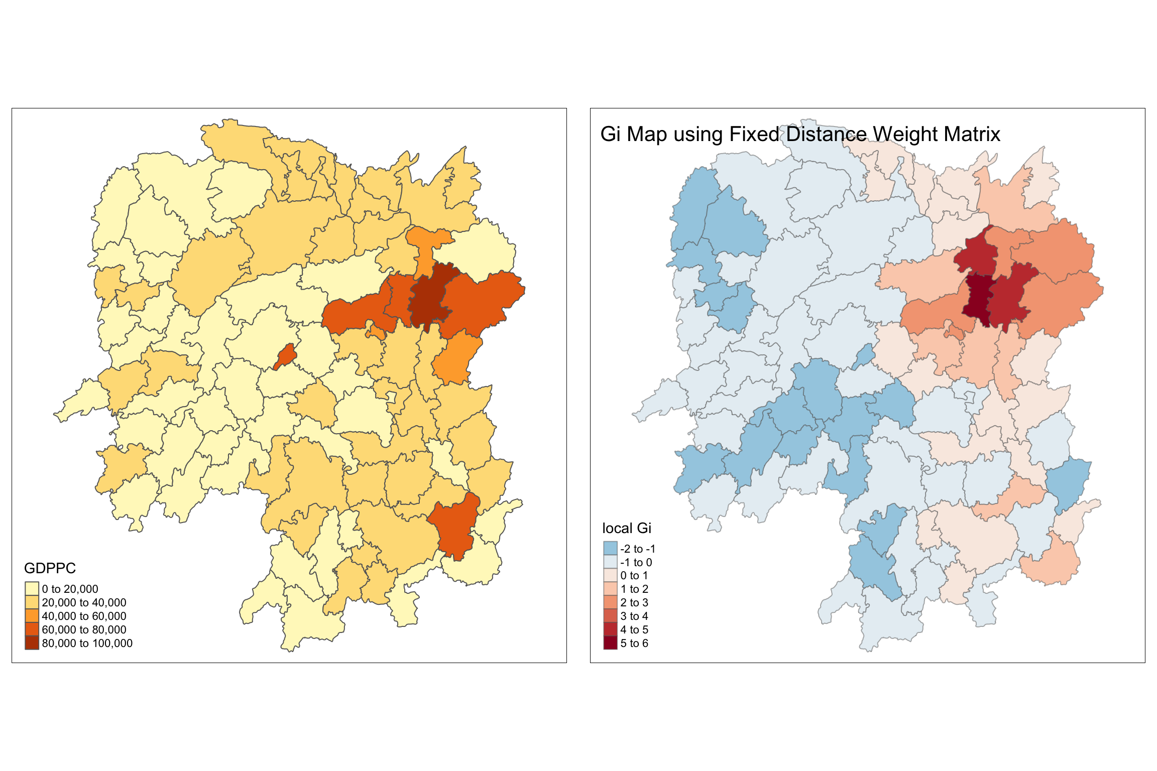
Note
Question: What statistical observation can you draw from the Gi map above?
see below with adaptive weight distance matrix viz.
11.3 Gi statistics using adaptive distance
Next, we use similar steps to compute the Gi values for GDPPC2012 by using an adaptive distance weight matrix (i.e knb_lw) and compare the methodology.
# adaptive distance
gdppc<- qtm(hunan, "GDPPC")

Gimap_ad <- tm_shape(hunan.gi) +
  tm_fill(col = "gstat_adaptive",
          style = "pretty",
          palette="-RdBu",
          title = "local Gi") +
  tm_borders(alpha = 0.5)+
  tm_layout(title = "Gi Map using Adaptive Distance Weight Matrix")


tmap_arrange(gdppc,
             Gimap_ad,
             asp=1,
             ncol=2)
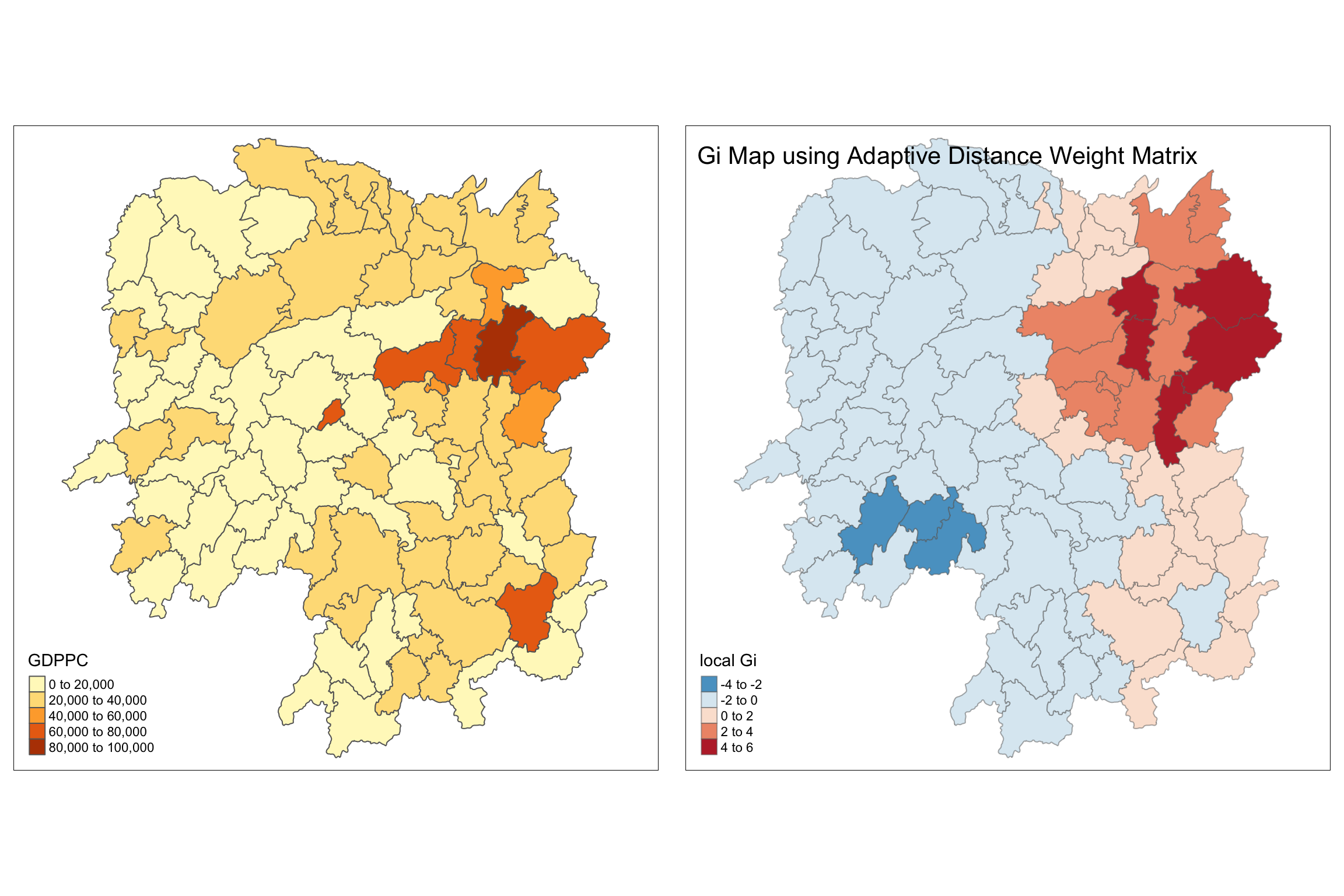
Note
Question: What statistical observation can you draw from the Gi maps (comparing between Fixed and Adaptive Weight matrix) above?
Both methods identify similar clusters in the central-eastern (hot spots), and western regions (cold spots), confirming consistent spatial patterns.
The fixed distance approach captures more localized clusters, while the adaptive distance approach reveals broader patterns (smoothing effect discussed above), adjusting dynamically to neighborhood density.
Also note that the range of legend is slightly different across the 2 methods.