pacman::p_load(sf, spNetwork, tmap, tidyverse)3A: Network Constrained Spatial Point Patterns Analysis
In this exercise, we will learn to use R and the
spNetwork package for analyzing network-constrained
spatial point patterns, focusing on kernel density estimation and
G- and K-function analysis.
1 Exercise 3A Reference
R for Geospatial Data Science and Analytics - 7 Network Constrained Spatial Point Patterns Analysis
2 Overview
Note
What is NetKDE and Why is it important? Network Constrained Kernel Density Estimation (NetKDE) is an advanced spatial analysis technique used to estimate the density of spatial events (such as crime incidents, traffic accidents, wildlife sightings, etc.) while accounting for the underlying network structure, such as roads, railways, or rivers. Unlike traditional Kernel Density Estimation (KDE), which assumes that events are distributed freely in a 2D plane, NetKDE restricts the analysis to a network, providing a more accurate representation when events are constrained to specific pathways or routes.
NetKDE provides a more realistic density estimation for data constrained to a network, avoiding misleading results that might arise from traditional KDE. For example, traffic accidents or crime hotspots along a road network are better analyzed using NetKDE since it restricts the analysis to the roads themselves.
Network constrained Spatial Point Patterns Analysis (NetSPAA) is a collection of spatial point patterns analysis methods special developed for analysing spatial point event occurs on or alongside network. The spatial point event can be locations of traffic accident or childcare centre for example. The network, on the other hand can be a road network or river network.
In this hands-on exercise, you are going to gain hands-on experience on using appropriate functions of spNetwork package:
- to derive network kernel density estimation (NKDE), and
- to perform network G-function and k-function analysis
3 Learning Outcome
- Understand and perform Network Constrained Spatial Point Patterns Analysis (NetSPAA) for events on networks (e.g., traffic accidents, childcare centers).
-
Use
spNetworkto derive network kernel density estimation (NKDE) for spatial analysis. - Conduct network G- and K-function analyses to test for complete spatial randomness (CSR).
-
Visualize geospatial data using
tmapfor interactive and high-quality mapping. -
Prepare data by importing geospatial datasets using the
sfpackage and managing CRS information. -
Use
lixelize_lines()to cut lines into lixels for NKDE analysis. -
Apply NKDE methods (
simple,discontinuous,continuous) to analyze point patterns on networks. - Visualize NKDE results by rescaling densities for effective mapping.
-
Perform CSR tests using the
kfunctions()fromspNetworkto analyze spatial interactions among events.
4 The Data
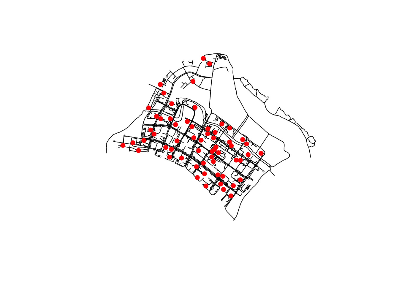
This study will analyze the spatial distribution of childcare centers in the Punggol planning area using the following geospatial datasets:
| Dataset | Description | Format |
|---|---|---|
| Punggol_St | Line feature data representing the road network within Punggol Planning Area. | ESRI Shapefile |
| Punggol_CC | Point feature data representing the location of childcare centers within Punggol Planning Area. | ESRI Shapefile |
5 Installing and Launching the R Packages
The following R packages will be used in this exercise:
| Package | Purpose | Use Case in Exercise |
|---|---|---|
| spNetwork | Provides functions for Spatial Point Patterns Analysis (e.g., KDE, K-function) on networks and spatial matrix building for spatial analysis. | Conducting spatial point pattern analysis and building spatial weights based on network distances. |
| sf | Offers functions to manage, process, and manipulate Simple Features for geospatial data handling. | Handling and processing geospatial data in Simple Features format. |
| tmap | Creates cartographic quality static and interactive maps using the Leaflet API. | Plotting high-quality static and interactive maps for spatial analysis. |
To install and load these packages, use the following code:
6 Import Data and Preparation
The code block below uses st_read() of
sf package to important Punggol_St and Punggol_CC
geospatial data sets into RStudio as sf data frames.
network <- st_read(dsn="data/geospatial",
layer="Punggol_St")Reading layer `Punggol_St' from data source
`/Users/walter/code/isss626/isss626-gaa/Hands-on_Ex/Hands-on_Ex03/data/geospatial'
using driver `ESRI Shapefile'
Simple feature collection with 2642 features and 2 fields
Geometry type: LINESTRING
Dimension: XY
Bounding box: xmin: 34038.56 ymin: 40941.11 xmax: 38882.85 ymax: 44801.27
Projected CRS: SVY21 / Singapore TMchildcare <- st_read(dsn="data/geospatial",
layer="Punggol_CC")Reading layer `Punggol_CC' from data source
`/Users/walter/code/isss626/isss626-gaa/Hands-on_Ex/Hands-on_Ex03/data/geospatial'
using driver `ESRI Shapefile'
Simple feature collection with 61 features and 1 field
Geometry type: POINT
Dimension: XYZ
Bounding box: xmin: 34423.98 ymin: 41503.6 xmax: 37619.47 ymax: 44685.77
z_range: zmin: 0 zmax: 0
Projected CRS: SVY21 / Singapore TM6.1 Examine Data Content
We can examine the structure of the output simple features data tables in RStudio. Alternatively, we can print basic information on the data as shown below.
networkSimple feature collection with 2642 features and 2 fields
Geometry type: LINESTRING
Dimension: XY
Bounding box: xmin: 34038.56 ymin: 40941.11 xmax: 38882.85 ymax: 44801.27
Projected CRS: SVY21 / Singapore TM
First 10 features:
LINK_ID ST_NAME geometry
1 116130894 PUNGGOL RD LINESTRING (36546.89 44574....
2 116130897 PONGGOL TWENTY-FOURTH AVE LINESTRING (36546.89 44574....
3 116130901 PONGGOL SEVENTEENTH AVE LINESTRING (36012.73 44154....
4 116130902 PONGGOL SEVENTEENTH AVE LINESTRING (36062.81 44197....
5 116130907 PUNGGOL CENTRAL LINESTRING (36131.85 42755....
6 116130908 PUNGGOL RD LINESTRING (36112.93 42752....
7 116130909 PUNGGOL CENTRAL LINESTRING (36127.4 42744.5...
8 116130910 PUNGGOL FLD LINESTRING (35994.98 42428....
9 116130911 PUNGGOL FLD LINESTRING (35984.97 42407....
10 116130912 EDGEFIELD PLNS LINESTRING (36200.87 42219....dim(network)[1] 2642 3str(network)Classes 'sf' and 'data.frame': 2642 obs. of 3 variables:
$ LINK_ID : num 1.16e+08 1.16e+08 1.16e+08 1.16e+08 1.16e+08 ...
$ ST_NAME : chr "PUNGGOL RD" "PONGGOL TWENTY-FOURTH AVE" "PONGGOL SEVENTEENTH AVE" "PONGGOL SEVENTEENTH AVE" ...
$ geometry:sfc_LINESTRING of length 2642; first list element: 'XY' num [1:2, 1:2] 36547 36559 44575 44614
- attr(*, "sf_column")= chr "geometry"
- attr(*, "agr")= Factor w/ 3 levels "constant","aggregate",..: NA NA
..- attr(*, "names")= chr [1:2] "LINK_ID" "ST_NAME"st_crs(network)Coordinate Reference System:
User input: SVY21 / Singapore TM
wkt:
PROJCRS["SVY21 / Singapore TM",
BASEGEOGCRS["SVY21",
DATUM["SVY21",
ELLIPSOID["WGS 84",6378137,298.257223563,
LENGTHUNIT["metre",1]]],
PRIMEM["Greenwich",0,
ANGLEUNIT["degree",0.0174532925199433]],
ID["EPSG",4757]],
CONVERSION["Singapore Transverse Mercator",
METHOD["Transverse Mercator",
ID["EPSG",9807]],
PARAMETER["Latitude of natural origin",1.36666666666667,
ANGLEUNIT["degree",0.0174532925199433],
ID["EPSG",8801]],
PARAMETER["Longitude of natural origin",103.833333333333,
ANGLEUNIT["degree",0.0174532925199433],
ID["EPSG",8802]],
PARAMETER["Scale factor at natural origin",1,
SCALEUNIT["unity",1],
ID["EPSG",8805]],
PARAMETER["False easting",28001.642,
LENGTHUNIT["metre",1],
ID["EPSG",8806]],
PARAMETER["False northing",38744.572,
LENGTHUNIT["metre",1],
ID["EPSG",8807]]],
CS[Cartesian,2],
AXIS["northing (N)",north,
ORDER[1],
LENGTHUNIT["metre",1]],
AXIS["easting (E)",east,
ORDER[2],
LENGTHUNIT["metre",1]],
USAGE[
SCOPE["Cadastre, engineering survey, topographic mapping."],
AREA["Singapore - onshore and offshore."],
BBOX[1.13,103.59,1.47,104.07]],
ID["EPSG",3414]]childcareSimple feature collection with 61 features and 1 field
Geometry type: POINT
Dimension: XYZ
Bounding box: xmin: 34423.98 ymin: 41503.6 xmax: 37619.47 ymax: 44685.77
z_range: zmin: 0 zmax: 0
Projected CRS: SVY21 / Singapore TM
First 10 features:
Name geometry
1 kml_10 POINT Z (36173.81 42550.33 0)
2 kml_99 POINT Z (36479.56 42405.21 0)
3 kml_100 POINT Z (36618.72 41989.13 0)
4 kml_101 POINT Z (36285.37 42261.42 0)
5 kml_122 POINT Z (35414.54 42625.1 0)
6 kml_161 POINT Z (36545.16 42580.09 0)
7 kml_172 POINT Z (35289.44 44083.57 0)
8 kml_188 POINT Z (36520.56 42844.74 0)
9 kml_205 POINT Z (36924.01 41503.6 0)
10 kml_222 POINT Z (37141.76 42326.36 0)dim(childcare)[1] 61 2str(childcare)Classes 'sf' and 'data.frame': 61 obs. of 2 variables:
$ Name : chr "kml_10" "kml_99" "kml_100" "kml_101" ...
$ geometry:sfc_POINT of length 61; first list element: 'XYZ' num 36174 42550 0
- attr(*, "sf_column")= chr "geometry"
- attr(*, "agr")= Factor w/ 3 levels "constant","aggregate",..: NA
..- attr(*, "names")= chr "Name"st_crs(childcare)Coordinate Reference System:
User input: SVY21 / Singapore TM
wkt:
PROJCRS["SVY21 / Singapore TM",
BASEGEOGCRS["SVY21",
DATUM["SVY21",
ELLIPSOID["WGS 84",6378137,298.257223563,
LENGTHUNIT["metre",1]]],
PRIMEM["Greenwich",0,
ANGLEUNIT["degree",0.0174532925199433]],
ID["EPSG",4757]],
CONVERSION["Singapore Transverse Mercator",
METHOD["Transverse Mercator",
ID["EPSG",9807]],
PARAMETER["Latitude of natural origin",1.36666666666667,
ANGLEUNIT["degree",0.0174532925199433],
ID["EPSG",8801]],
PARAMETER["Longitude of natural origin",103.833333333333,
ANGLEUNIT["degree",0.0174532925199433],
ID["EPSG",8802]],
PARAMETER["Scale factor at natural origin",1,
SCALEUNIT["unity",1],
ID["EPSG",8805]],
PARAMETER["False easting",28001.642,
LENGTHUNIT["metre",1],
ID["EPSG",8806]],
PARAMETER["False northing",38744.572,
LENGTHUNIT["metre",1],
ID["EPSG",8807]]],
CS[Cartesian,2],
AXIS["northing (N)",north,
ORDER[1],
LENGTHUNIT["metre",1]],
AXIS["easting (E)",east,
ORDER[2],
LENGTHUNIT["metre",1]],
USAGE[
SCOPE["Cadastre, engineering survey, topographic mapping."],
AREA["Singapore - onshore and offshore."],
BBOX[1.13,103.59,1.47,104.07]],
ID["EPSG",3414]]7 Visualising Geospatial Data
To visualise geospatial data, we can use
plot()
from base R. Alternatively, we can visualise the geospatial data
with high cartographic quality and interactive manner using the
tmap package.
8 Network Constrained KDE (NKDE) Analysis using spNetwork
In this section, we will perform NKDE analysis by using appropriate functions provided in spNetwork package.
8.1 Preparing the Lixels Objects
Before computing NKDE, the SpatialLines object need to be cut into lixels with a specified minimal distance. This task can be performed by using with lixelize_lines() of spNetwork as shown in the code block below.
lixels <- lixelize_lines(lines=network,
lx_length=700,
mindist = 375)Note
Arguments
-
lines: The sf object with linestring geometry type to modify
lx_length: The length of a lixel
-
mindist: The minimum length of a lixel. After cut, if the length of the final lixel is shorter than the minimum distance, then it is added to the previous lixel. if NULL, then mindist = maxdist/10. Note that the segments that are already shorter than the minimum distance are not modified
There is another function called
lixelize_lines.mc() which provide multicore
support.
8.2 Generating Line Centre Points
Next, we will use lines_center() of
spNetwork to generate a SpatialPointsDataFrame
(i.e. samples) with line centre points.
samples <- lines_center(lixels)The points are located at center of the line based on the length of the line.
8.3 Performing NKDE
To compute the NKDE:
Note
-
spNetwork supports various kernel methods, including
quartic, triangle, gaussian, scaled gaussian, tricube, cosine, triweight, epanechnikov, or uniform. In this case,quartickernel is used. -
method argument indicates that
simplemethod is used to calculate the NKDE. Currently, spNetwork support three popular methods, they are:- method=“simple”. This first method was presented by Xie et al. (2008) and proposes an intuitive solution. The distances between events and sampling points are replaced by network distances, and the formula of the kernel is adapted to calculate the density over a linear unit instead of an areal unit.
- method=“discontinuous”. The method is proposed by Okabe et al (2008), which equally “divides” the mass density of an event at intersections of lixels.
- method=“continuous”. If the discontinuous method is unbiased, it leads to a discontinuous kernel function which is a bit counter-intuitive. Okabe et al (2008) proposed another version of the kernel, that divide the mass of the density at intersection but adjusts the density before the intersection to make the function continuous.
For more info, refer to the user guide of spNetwork package.
8.4 Visualising NKDE
To visualise the NKDE values, we have to perform a few preparation steps.
- Insert the computed density values (i.e. densities) into samples and lixels objects as density field.
samples$density <- densities
lixels$density <- densities- rescale the density values if required.
Since svy21 projection system is in meter, the computed density values are very small i.e. 0.0000005. We should rescale the density values from number of events per meter to number of events per kilometer.
samples$density <- samples$density*1000
lixels$density <- lixels$density*1000- Use tmap to plot interactive map
tmap_mode('view')
tm_shape(lixels)+
tm_lines(col="density")+
tm_shape(childcare)+
tm_dots()Note
Road segments with relatively higher density of childcare centres is shown in darker color (refer to legend). Road segments with relatively lower density of childcare centre is shown in lighter color.
9 Network Constrained G- and K-Function Analysis
In this section, we are going to perform Complete Spatial Randomness (CSR) test by using kfunctions() of spNetwork package.
The CSR test is based on the assumption of the binomial point process which implies the hypothesis that the childcare centres are randomly and independently distributed over the street network.
Null Hypothesis (\(H_0\)): The observed spatial point events (i.e., distribution of childcare centres) exhibit a uniform distribution over a street network in Punggol Planning Area.
If this hypothesis is rejected, we may infer that the distribution of childcare centres are spatially interacting and dependent on each other; as a result, they may form non-random patterns.
# set seed for reproducibility
set.seed(1234)
kfun_childcare <- kfunctions(network,
childcare,
start = 0,
end = 1000,
step = 50,
width = 50,
nsim = 39,
resolution = 50,
verbose = FALSE,
conf_int = 0.05)Note
Explanation on Arguments used
-
lines: A SpatialLinesDataFrame with sampling points. -
points: A SpatialPointsDataFrame representing points on the network. -
start: Start value for evaluating the k and g functions. -
end: Last value for evaluating the k and g functions. -
step: Jump between two evaluations of the k and g functions. -
width: Width of each donut for the g-function. -
nsim: Number of Monte Carlo simulations (39 simulations in this example, more simulation may be required for inference). -
resolution: Resolution for simulating random points on the network. -
conf_int: Width of the confidence interval (default = 0.05). - For additional arguments, refer to the user guide of the spNetwork package.
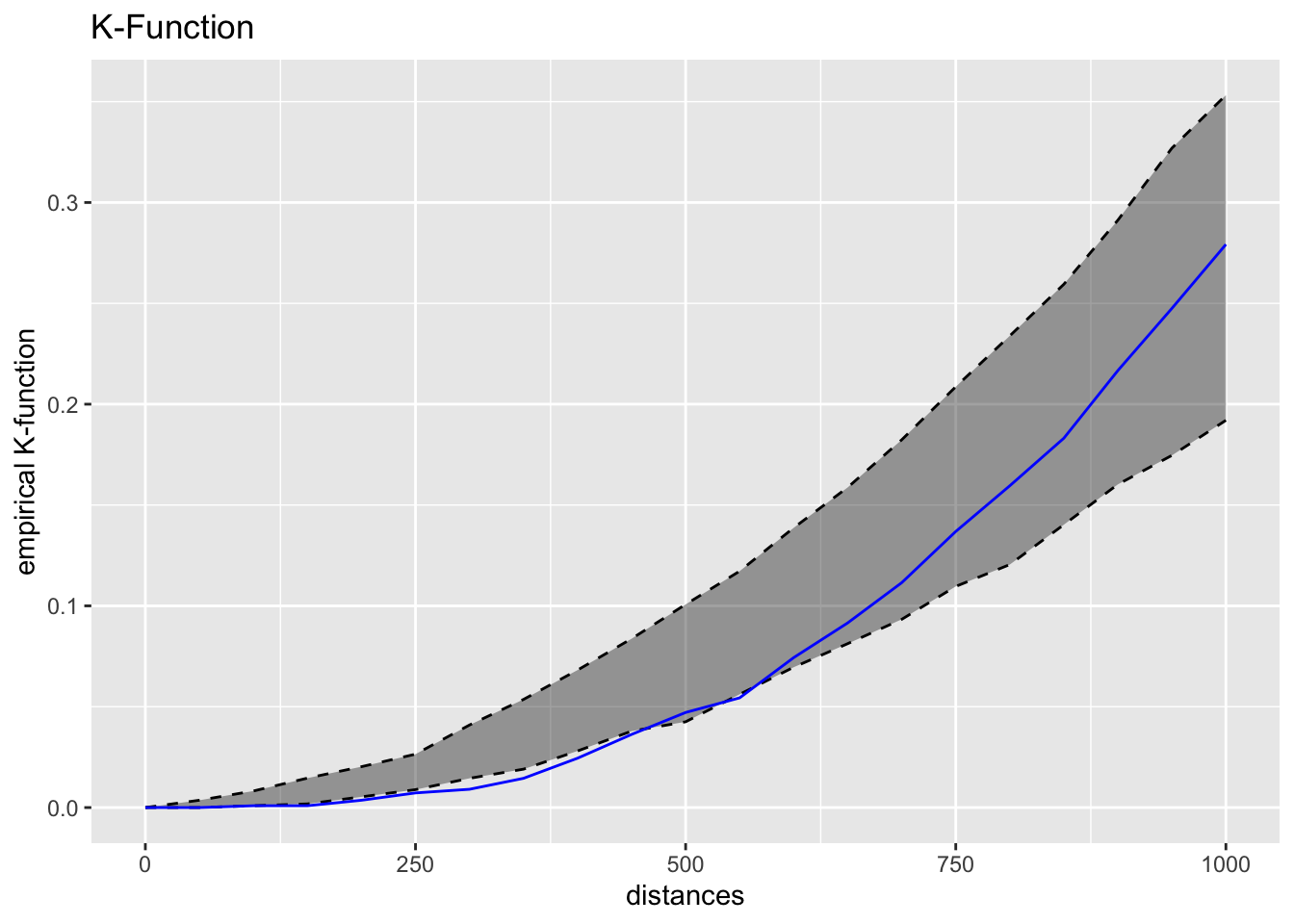
We can visualise the ggplot2 object of k-function by using the code chunk below.
kfun_childcare$plotk +
labs(title ="K-Function")
Note
Intepretation of kfunctions() outputs
-
plotk: A ggplot2 object representing the values of the k-function -
plotg: A ggplot2 object representing the values of the g-function -
values: A DataFrame with the values used to build the plots
see kfunctions function - RDocumentation
Intepretation of the graph output
The blue line is the empirical network K-function of the childcare centres in Punggol planning area. The gray envelope represents the results of the 39 simulations in the interval 2.5% - 97.5%.
Since the blue line between the distance of 250m-400m are below the gray area, we can infer that the childcare centres in Punggol planning area resemble regular pattern at the distance of 250m-400m.