pacman::p_load(tmap, sf, DT, stplanr, tidyverse, knitr)10A: Processing and Visualising Flow Data
In this exercise, we will explore the concept of spatial interaction, and learn how to build an OD (origin/destination) matrix.
1 Exercise 10A Reference
R for Geospatial Data Science and Analytics - 15 Processing and Visualising Flow Data
2 Overview
In this exercise, we will explore the concept of spatial interaction, and learn how to build an OD (origin/destination) matrix.
Spatial interaction represent the flow of people, material, or information between locations in geographical space. It encompasses everything from freight shipments, energy flows, and the global trade in rare antiquities, to flight schedules, rush hour woes, and pedestrian foot traffic.
An OD matrix, or spatial interaction matrix, represents each spatial interaction as a discrete origin/destination pair, where each pair corresponds to a cell in the matrix; the rows denote the locations (centroids) of origin, and the columns represent the locations (centroids) of destination.
3 Learning Outcome
- Import and extract OD data for a selected time interval.
- Import and save geospatial data (bus stops and planning subzones) into sf tibble data frame objects.
- Populate planning subzone codes into bus stops sf tibble data frames.
- Construct desire lines geospatial data from the OD data.
- Visualize passenger volume by origin and destination bus stops using the desire lines data.
4 The Data
The following datasets will be used in this exercise:
| Data Set | Description | Format |
|---|---|---|
| Passenger Volume by Origin Destination Bus Stops | OD data set representing the volume of passengers traveling between bus stops. | CSV |
| BusStop | Geospatial data providing the locations of bus stops as of the last quarter of 2022. | ESRI Shapefile |
| MPSZ-2019 | Geospatial data providing the sub-zone boundary of the URA Master Plan 2019. | ESRI Shapefile |
5 Installing and Launching the R Packages
The following R packages will be used in this exercise:
| Package | Purpose | Use Case in Exercise |
|---|---|---|
| sf | Handles vector-based geospatial data. | Importing, processing, and transforming geospatial data, such as bus stop locations and sub-zone boundaries. |
| tidyverse | A collection of packages for data science tasks such as data manipulation, visualization, and modeling. | Importing and wrangling OD and geospatial data, and visualizing analysis outputs. |
| tmap | Creates static and interactive thematic maps using cartographic quality elements. | Visualizing passenger flows and geographic clusters in a cartographic format. |
| stplanr | Provides functions for transport planning and modeling. | Creating geographic desire lines from OD data and solving transport-related problems. |
| DT | Provides an R interface to the JavaScript library DataTables for interactive table display. | Displaying data tables in an interactive format within the HTML output. |
To install and load these packages, use the following code:
6 Preparing the Flow Data
6.1 Importing the OD data
First, we import the
Passenger Volume by Origin Destination Bus Stops dataset
using read_csv() from the
readr package.
odbus <- read_csv("data/aspatial/origin_destination_bus_202408.csv")
glimpse(odbus)
Rows: 5,760,081
Columns: 7
$ YEAR_MONTH <chr> "2024-08", "2024-08", "2024-08", "2024-08", "2024-…
$ DAY_TYPE <chr> "WEEKENDS/HOLIDAY", "WEEKENDS/HOLIDAY", "WEEKENDS/…
$ TIME_PER_HOUR <dbl> 18, 7, 19, 9, 5, 12, 23, 15, 12, 13, 7, 9, 17, 15,…
$ PT_TYPE <chr> "BUS", "BUS", "BUS", "BUS", "BUS", "BUS", "BUS", "…
$ ORIGIN_PT_CODE <chr> "76201", "10351", "76061", "14271", "54581", "1008…
$ DESTINATION_PT_CODE <chr> "76079", "13201", "75371", "07021", "66471", "1007…
$ TOTAL_TRIPS <dbl> 6, 7, 1, 2, 1, 145, 2, 78, 2, 1, 3, 1, 2, 3, 5, 3,…
odbus tibble data frame shows that the values in
ORIGIN_PT_CODE and
DESTINATON_PT_CODE are in character data type, we
will convert themm into factor data type.
odbus$ORIGIN_PT_CODE <- as.factor(odbus$ORIGIN_PT_CODE)
odbus$DESTINATION_PT_CODE <- as.factor(odbus$DESTINATION_PT_CODE)
glimpse(odbus)
Rows: 5,760,081
Columns: 7
$ YEAR_MONTH <chr> "2024-08", "2024-08", "2024-08", "2024-08", "2024-…
$ DAY_TYPE <chr> "WEEKENDS/HOLIDAY", "WEEKENDS/HOLIDAY", "WEEKENDS/…
$ TIME_PER_HOUR <dbl> 18, 7, 19, 9, 5, 12, 23, 15, 12, 13, 7, 9, 17, 15,…
$ PT_TYPE <chr> "BUS", "BUS", "BUS", "BUS", "BUS", "BUS", "BUS", "…
$ ORIGIN_PT_CODE <fct> 76201, 10351, 76061, 14271, 54581, 10089, 67231, 5…
$ DESTINATION_PT_CODE <fct> 76079, 13201, 75371, 07021, 66471, 10079, 67179, 5…
$ TOTAL_TRIPS <dbl> 6, 7, 1, 2, 1, 145, 2, 78, 2, 1, 3, 1, 2, 3, 5, 3,…6.2 Extracting the Study Data
For the purpose of this exercise, we extract commuting flows on weekdays between 6 and 9 a.m. and sum the trips.
The table below shows the head content of odbus6_9:
datatable(head(odbus6_9, 10))6.3 Saving and loading the data
We save the filtered data for future use in RDS format.
write_rds(odbus6_9, "data/rds/odbus6_9.rds")
odbus6_9 <- read_rds("data/rds/odbus6_9.rds")
7 Working with Geospatial Data
For this exercise, two geospatial datasets will be used:
- BusStop: Contains the locations of bus stops as of Q4 2022.
- MPSZ-2019: Provides the sub-zone boundaries from the URA Master Plan 2019.
Both datasets are in ESRI shapefile format.
7.1 Importing Geospatial Data
The code below imports the geospatial data:
busstop <- st_read(dsn = "data/geospatial", layer = "BusStop") %>%
  st_transform(crs = 3414)
Reading layer `BusStop' from data source
`/Users/walter/code/isss626/isss626-gaa/Hands-on_Ex/Hands-on_Ex10/data/geospatial'
using driver `ESRI Shapefile'
Simple feature collection with 5166 features and 3 fields
Geometry type: POINT
Dimension: XY
Bounding box: xmin: 3970.122 ymin: 26482.1 xmax: 48285.52 ymax: 52983.82
Projected CRS: SVY21mpsz <- st_read(dsn = "data/geospatial", layer = "MPSZ-2019") %>%
st_transform(crs = 3414)Reading layer `MPSZ-2019' from data source
`/Users/walter/code/isss626/isss626-gaa/Hands-on_Ex/Hands-on_Ex10/data/geospatial'
using driver `ESRI Shapefile'
Simple feature collection with 332 features and 6 fields
Geometry type: MULTIPOLYGON
Dimension: XY
Bounding box: xmin: 103.6057 ymin: 1.158699 xmax: 104.0885 ymax: 1.470775
Geodetic CRS: WGS 84mpsz <- write_rds(mpsz, "data/rds/mpsz.rds")8 Geospatial Data Wrangling
8.1 Combining BusStop and MPSZ
The code below joins the planning subzone codes from
mpsz to the bus stops in busstop:
busstop_mpsz <- st_intersection(busstop, mpsz) %>%
  select(BUS_STOP_N, SUBZONE_C) %>%
st_drop_geometry()datatable(head(busstop_mpsz, 10))Note
-
st_intersection()performs a point-and-polygon overlay. -
select()keeps onlyBUS_STOP_NandSUBZONE_Cfields. - Five bus stops outside Singapore are excluded.
Save the result as an RDS file:
write_rds(busstop_mpsz, "data/rds/busstop_mpsz.rds")
Next, append the subzone codes to the
odbus6_9 dataset:
od_data <- left_join(odbus6_9, busstop_mpsz, by = c("ORIGIN_PT_CODE" = "BUS_STOP_N")) %>%
  rename(ORIGIN_BS = ORIGIN_PT_CODE, ORIGIN_SZ = SUBZONE_C, DESTIN_BS = DESTINATION_PT_CODE)
Check for duplicate records:
duplicate <- od_data %>%
  group_by_all() %>%
  filter(n() > 1) %>%
  ungroup()

duplicate
# A tibble: 1,464 × 4
ORIGIN_BS DESTIN_BS TRIPS ORIGIN_SZ
<chr> <fct> <dbl> <chr>
1 09047 02029 2 ORSZ02
2 09047 02029 2 ORSZ02
3 09047 02049 49 ORSZ02
4 09047 02049 49 ORSZ02
5 09047 02089 46 ORSZ02
6 09047 02089 46 ORSZ02
7 09047 02151 95 ORSZ02
8 09047 02151 95 ORSZ02
9 09047 02161 35 ORSZ02
10 09047 02161 35 ORSZ02
# ℹ 1,454 more rowsSince duplicates exist, we will remove them:
Now, append the destination subzone codes:
Finally, save the cleaned data:
write_rds(od_data_fii, "data/rds/od_data_fii.rds")
od_data_fii <- read_rds("data/rds/od_data_fii.rds")
9 Visualising Spatial Interaction
In this section, we will prepare a desire line by using stplanr package.
9.1 Removing Intra-Zonal Flows
We will exclude flows within the same zone to focus on inter-zonal flows. The code below removes these intra-zonal flows:
od_data_fij <- od_data[od_data$ORIGIN_SZ != od_data$DESTIN_SZ,]Tip
The comma in the code
od_data1 <- od_data[od_data$ORIGIN_SZ !=
                    od_data$DESTIN_SZ,]
is crucial because it specifies that you are subsetting the
rows of the data frame based on a condition, while keeping all
the columns.
Save the result for future use:
write_rds(od_data_fij, "data/rds/od_data_fij.rds")od_data_fij <- read_rds("data/rds/od_data_fij.rds")9.2 Creating Desire Lines
Note
Desire lines are used to illustrate on a map the flows of people or goods from point to point based on the values from a matrix.
Next, we use od2line() from the
stplanr package to generate desire lines:
flowLine <- od2line(flow = od_data_fij,
                    zones = mpsz,
                    zone_code = "SUBZONE_C")

flowLine
Simple feature collection with 20625 features and 3 fields
Geometry type: LINESTRING
Dimension: XY
Bounding box: xmin: 5105.594 ymin: 25813.33 xmax: 46654.41 ymax: 49552.79
Projected CRS: SVY21 / Singapore TM
First 10 features:
ORIGIN_SZ DESTIN_SZ MORNING_PEAK geometry
1 AMSZ01 AMSZ02 10895 LINESTRING (29501.77 39419....
2 AMSZ01 AMSZ03 15626 LINESTRING (29501.77 39419....
3 AMSZ01 AMSZ04 2865 LINESTRING (29501.77 39419....
4 AMSZ01 AMSZ05 8166 LINESTRING (29501.77 39419....
5 AMSZ01 AMSZ06 2309 LINESTRING (29501.77 39419....
6 AMSZ01 AMSZ07 1446 LINESTRING (29501.77 39419....
7 AMSZ01 AMSZ08 2572 LINESTRING (29501.77 39419....
8 AMSZ01 AMSZ09 2380 LINESTRING (29501.77 39419....
9 AMSZ01 AMSZ10 287 LINESTRING (29501.77 39419....
10 AMSZ01 AMSZ11 741 LINESTRING (29501.77 39419....Save the generated desire lines:
write_rds(flowLine, "data/rds/flowLine.rds")

flowLine <- read_rds("data/rds/flowLine.rds")
9.3 Filtering High-Volume Flows
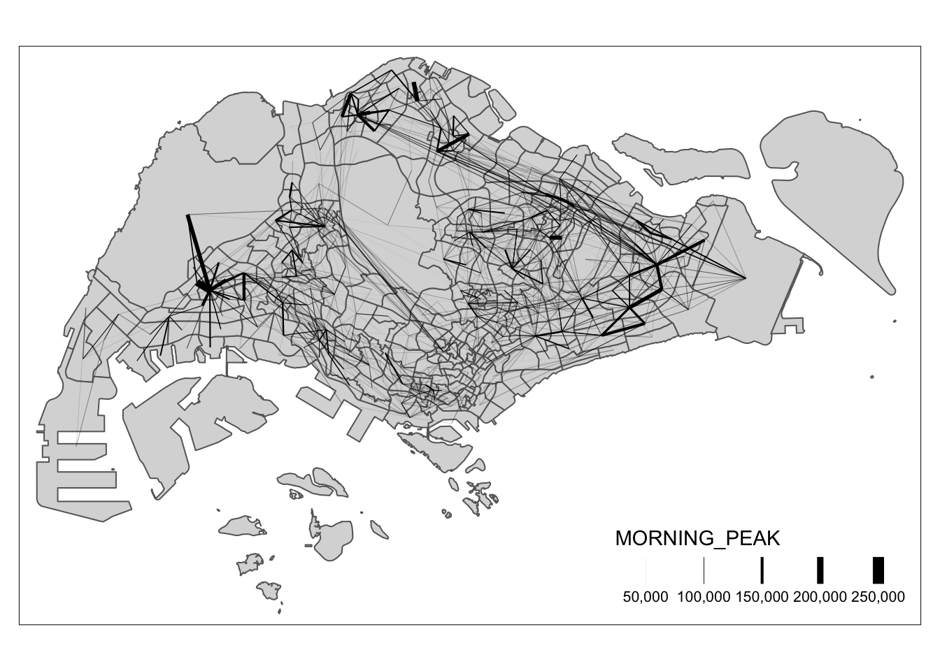
To simplify the visual output and focus on significant flows, we filter for high-volumes flows.
summary(flowLine$MORNING_PEAK) Min. 1st Qu. Median Mean 3rd Qu. Max.
1.0 16.0 84.0 993.9 429.0 218070.0 For example, we can visualize flow greater than or equal to 2000 as shown below.