4A: Spatial Weights and Applications

In this exercise, we will learn to compute spatial weights, visualize spatial distributions, and create spatially lagged variables using various functions from R packages such as sf,spdep, and tmap.

Author

Teng Kok Wai (Walter)

Published

September 8, 2024

Modified

September 27, 2024

1 Exercise 4A Reference

R for Geospatial Data Science and Analytics - 8 Spatial Weights and Applications

2 Overview

In this exercise, we will learn to compute spatial weights, visualize spatial distributions, and create spatially lagged variables using various functions from R packages such as sf, spdep, and tmap.

3 Learning Outcome

Import geospatial data using functions from the sf package.
Import CSV data using functions from the readr package.
Perform relational joins using functions from the dplyr package.
Compute spatial weights with functions from the spdep package.
Calculate spatially lagged variables using functions from the spdep package.

4 The Data

The following 2 datasets will be used in this exercise.

Data Set	Description	Format
Hunan county boundary layer	Geospatial data set representing the county boundaries of Hunan	ESRI Shapefile
Hunan_2012.csv	Contains selected local development indicators for Hunan in 2012	CSV

5 Installing and Loading the R Packages

The following R packages will be used in this exercise:

Package	Purpose	Use Case in Exercise
sf	Imports, manages, and processes vector-based geospatial data.	Handling vector geospatial data such as the Hunan county boundary layer in shapefile format.
spdep	Provides functions for spatial dependence analysis, including spatial weights and spatial autocorrelation.	Computing spatial weights and creating spatially lagged variables.
tmap	Creates static and interactive thematic maps using cartographic quality elements.	Visualizing regional development indicators and plotting maps showing spatial relationships and patterns.
tidyverse	A collection of packages for data science tasks such as data manipulation, visualization, and modeling.	Importing CSV files, wrangling data, and performing relational joins.
knitr	Enables dynamic report generation and integration of R code with documents.	Formatting output, creating tables, and generating reports for the exercise.

To install and load these packages, use the following code:

pacman::p_load(sf, spdep, tmap, tidyverse, knitr)

6 Import Data and Preparation

In this section, we will perform 3 necessary steps to prepare the data for analysis.

6.1 Import Geospatial Shapefile

Firstly, we will use st_read() of sf package to import Hunan shapefile into R. The imported shapefile will be simple features Object of sf.

hunan <- st_read(dsn = "data/geospatial", 
                 layer = "Hunan")

Reading layer `Hunan' from data source
  `/Users/walter/code/isss626/isss626-gaa/Hands-on_Ex/Hands-on_Ex04/data/geospatial'
  using driver `ESRI Shapefile'
Simple feature collection with 88 features and 7 fields
Geometry type: POLYGON
Dimension:     XY
Bounding box:  xmin: 108.7831 ymin: 24.6342 xmax: 114.2544 ymax: 30.12812
Geodetic CRS:  WGS 84

dim(hunan)

[1] 88  8

6.2 Import Aspatial csv File

Next, we will import Hunan_2012.csv into R by using read_csv() of readr package. The output is R dataframe class.

hunan2012 <- read_csv("data/aspatial/Hunan_2012.csv")

dim(hunan2012)

[1] 88 29

6.3 Perform Relational Join

Before we perform relational join, let’s observe the columns in each dataset and only select the columns that we need.

hunan columns:

print(colnames(hunan))

[1] "NAME_2"     "ID_3"       "NAME_3"     "ENGTYPE_3"  "Shape_Leng"
[6] "Shape_Area" "County"     "geometry"

hunan2012 columns:

print(colnames(hunan2012))

 [1] "County"      "City"        "avg_wage"    "deposite"    "FAI"
 [6] "Gov_Rev"     "Gov_Exp"     "GDP"         "GDPPC"       "GIO"
[11] "Loan"        "NIPCR"       "Bed"         "Emp"         "EmpR"
[16] "EmpRT"       "Pri_Stu"     "Sec_Stu"     "Household"   "Household_R"
[21] "NOIP"        "Pop_R"       "RSCG"        "Pop_T"       "Agri"
[26] "Service"     "Disp_Inc"    "RORP"        "ROREmp"

After merging:

hunan_joined <- left_join(hunan,hunan2012)
print(colnames(hunan_joined))

 [1] "NAME_2"      "ID_3"        "NAME_3"      "ENGTYPE_3"   "Shape_Leng"
 [6] "Shape_Area"  "County"      "City"        "avg_wage"    "deposite"
[11] "FAI"         "Gov_Rev"     "Gov_Exp"     "GDP"         "GDPPC"
[16] "GIO"         "Loan"        "NIPCR"       "Bed"         "Emp"
[21] "EmpR"        "EmpRT"       "Pri_Stu"     "Sec_Stu"     "Household"
[26] "Household_R" "NOIP"        "Pop_R"       "RSCG"        "Pop_T"
[31] "Agri"        "Service"     "Disp_Inc"    "RORP"        "ROREmp"
[36] "geometry"

Then only select the columns that we need:

hunan <- hunan_joined %>%
  select(1:4, 7, 15)

print(colnames(hunan))

[1] "NAME_2"    "ID_3"      "NAME_3"    "ENGTYPE_3" "County"    "GDPPC"
[7] "geometry"

In the code above, we use the left_join() function to merge the hunan SpatialPolygonsDataFrame with the hunan2012 dataframe. The join is based on the column named County, which is common to both datasets. This allows us to match rows by their corresponding counties.

After the join, the select() function is used to retain a subset of columns from the merged dataset. We can briefly observe the joined output below.

head(hunan)

Simple feature collection with 6 features and 6 fields
Geometry type: POLYGON
Dimension:     XY
Bounding box:  xmin: 110.4922 ymin: 28.61762 xmax: 112.3013 ymax: 30.12812
Geodetic CRS:  WGS 84
   NAME_2  ID_3  NAME_3   ENGTYPE_3  County GDPPC
1 Changde 21098 Anxiang      County Anxiang 23667
2 Changde 21100 Hanshou      County Hanshou 20981
3 Changde 21101  Jinshi County City  Jinshi 34592
4 Changde 21102      Li      County      Li 24473
5 Changde 21103   Linli      County   Linli 25554
6 Changde 21104  Shimen      County  Shimen 27137
                        geometry
1 POLYGON ((112.0625 29.75523...
2 POLYGON ((112.2288 29.11684...
3 POLYGON ((111.8927 29.6013,...
4 POLYGON ((111.3731 29.94649...
5 POLYGON ((111.6324 29.76288...
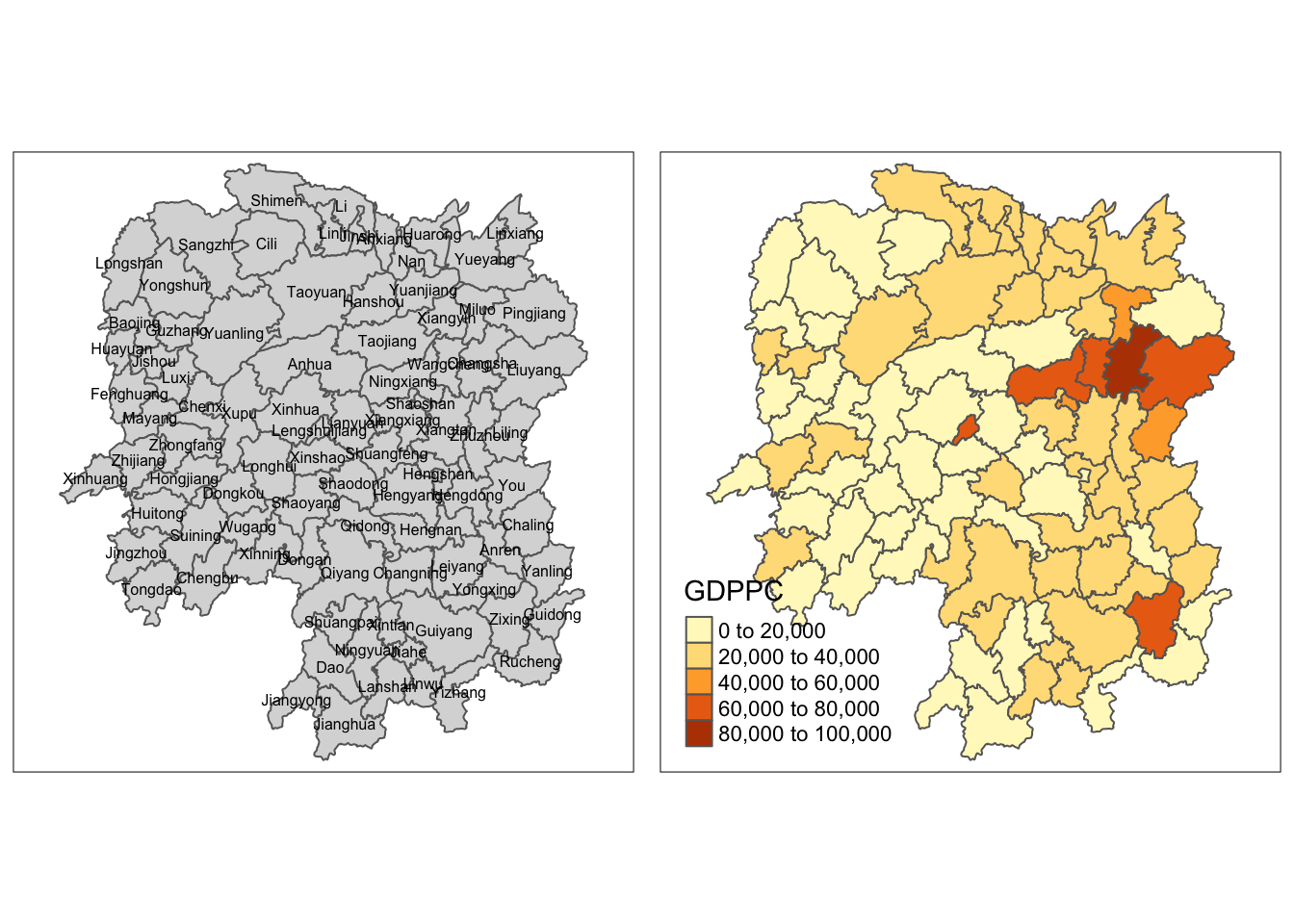
6 POLYGON ((110.8825 30.11675...

7 Visualising Regional Development Indicator

To visualize the regional development indicator, we can prepare a base map and a choropleth map to show the distribution of GDPPC 2012 (GDP per capita) by using qtm() of tmap package.

basemap <- tm_shape(hunan) +
  tm_polygons() +
  tm_text("NAME_3", size=0.5)

gdppc <- qtm(hunan, "GDPPC")
tmap_arrange(basemap, gdppc, asp=1, ncol=2)

Note

Intepretation The choropleth map on the right visualizes the distribution of GDP per capita (GDPPC) for the year 2012 across the different counties in Hunan.

The counties are shaded in varying colors, ranging from light to dark, to represent different GDP per capita ranges. Darker shades indicate higher GDP per capita values, while lighter shades represent lower values. This visualization helps to identify regional economic disparities and highlights areas with higher or lower economic activity within Hunan province.

For example, we can observe that Changsha has the highest GDP per capital values in the Hunan region.

8 Computing Contiguity Spatial Weights

In this section, we will use poly2nb() of spdep package to compute contiguity weight matrices for the study area. This function builds a neighbours list based on regions with contiguous boundaries.

Note

Contiguity means that two spatial units share a common border of non-zero length.

Operationally, we can further distinguish between a rook and a queen criterion of contiguity, in analogy to the moves allowed for the such-named pieces on a chess board.

The rook criterion defines neighbors by the existence of a common edge between two spatial units. The queen criterion is somewhat more encompassing and defines neighbors as spatial units sharing a common edge or a common vertex.

Using poly2nb() we can use the queen flag to toggle between queen and rook criteria.

For more info, see Chapter 6 Contiguity-Based Spatial Weights | Hands-On Spatial Data Science with R

The number of neighbors according to the queen criterion will always be at least as large as for the rook criterion.

First, we will compute the Queen contiguity weight matrix.

wm_q <- poly2nb(hunan, queen=TRUE)
summary(wm_q)

Neighbour list object:
Number of regions: 88
Number of nonzero links: 448
Percentage nonzero weights: 5.785124
Average number of links: 5.090909
Link number distribution:

 1  2  3  4  5  6  7  8  9 11
 2  2 12 16 24 14 11  4  2  1
2 least connected regions:
30 65 with 1 link
1 most connected region:
85 with 11 links

wm_r <- poly2nb(hunan, queen=FALSE)
summary(wm_r)

Neighbour list object:
Number of regions: 88
Number of nonzero links: 440
Percentage nonzero weights: 5.681818
Average number of links: 5
Link number distribution:

 1  2  3  4  5  6  7  8  9 10
 2  2 12 20 21 14 11  3  2  1
2 least connected regions:
30 65 with 1 link
1 most connected region:
85 with 10 links

Note

Intepretation of Summary Reports

Both reports shows that there are 88 area units in Hunan.
As expected, the total number of links (neighbor relationships) is slightly higher for the queen criterion (448) than for the rook criterion (440).
Based on both criteria, the most connected region is Region 85 with 11 links (using Queen criteria) and 10 links (using Rook criteria)
Similarly, based on both criteria, the least connected region is Region 30 and 65 with 1 links (using Queen and Rook criteria)

For each polygon in the polygon object, wm_q and wm_r lists all neighboring polygons. For example, we can identify the most connected region.

cat("The most connected county is", hunan$County[85])

The most connected county is Taoyuan

To reveal the county names of the neighboring polygons, we can do the following:

neighbour_counties <- wm_q[[85]]
print(neighbour_counties)

 [1]  1  2  3  5  6 32 56 57 69 75 78

cat("Using Queen's method, the neighbours of ", hunan$County[85]," is", hunan$NAME_3[neighbour_counties])

Using Queen's method, the neighbours of  Taoyuan  is Anxiang Hanshou Jinshi Linli Shimen Yuanling Anhua Nan Cili Sangzhi Taojiang

We can also retrieve the GDPPC of these counties:

hunan$GDPPC[neighbour_counties]

 [1] 23667 20981 34592 25554 27137 24194 14567 21311 18714 14624 19509

The printed output above shows that the GDPPC of Taoyuan’s neighbouring counties.

To display the complete weight matrix, we can use str().

str(wm_q)

9 Visualising Contiguity Weights

To create a connectivity graph, we need points that represent each polygon, and we’ll draw lines to connect neighboring points. Since we’re working with polygons, we first need to find their central points, called centroids. We’ll calculate these centroids using the sf package before creating the connectivity graph.

Getting Latitude and Longitude of Polygon Centroids

To make the connectivity graph, we must first obtain the points (centroids) for each polygon. This is more than just running st_centroid on our spatial object (us.bound). We need to store the coordinates in a separate data frame.

We’ll use a mapping function to achieve this. The mapping function applies a specific function to each element in a vector and returns a vector of the same length. In this case, our input vector will be the geometry column of us.bound, and the function will be st_centroid. We’ll use the map_dbl function from the purrr package to do this.

For longitude, we access the first coordinate value using [[1]], and for latitude, we access the second coordinate value using [[2]].

longitude <- map_dbl(hunan$geometry, ~st_centroid(.x)[[1]])
latitude <- map_dbl(hunan$geometry, ~st_centroid(.x)[[2]])

Then, we use cbind() to combine longitude and lattude into the same object.

coords <- cbind(longitude, latitude)

To verify that, the data is formatted correctly, we can observe the first few instances.

head(coords)

     longitude latitude
[1,]  112.1531 29.44362
[2,]  112.0372 28.86489
[3,]  111.8917 29.47107
[4,]  111.7031 29.74499
[5,]  111.6138 29.49258
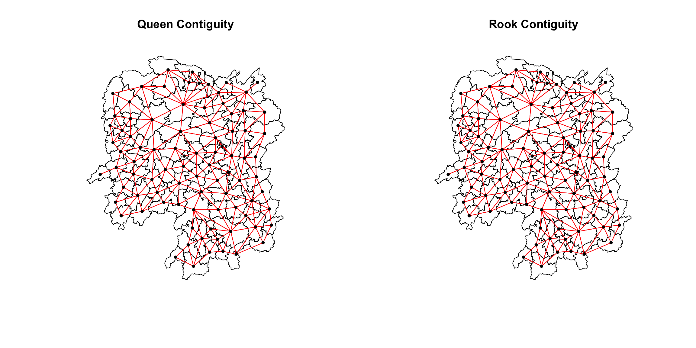
[6,]  111.0341 29.79863

To plot the continguity-based neighbours map, we can do the following:

par(mfrow=c(1,2))

plot(hunan$geometry, 
     main="Queen Contiguity")
plot(wm_q, 
     coords, 
     pch = 19, 
     cex = 0.6, 
     add = TRUE, 
     col= "red")

plot(hunan$geometry, 
     main="Rook Contiguity")
plot(wm_r, 
     coords, 
     pch = 19, 
     cex = 0.6, 
     add = TRUE, 
     col = "red")

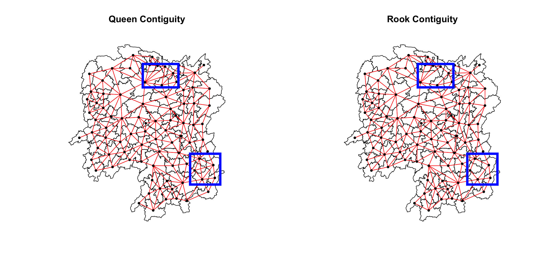::: callout-note As observed from the previous sections, we understand that more links will be formed with the Queen’s method. This is evident in the plot above.Some of these differences has been marked with blue boxes for better visualization. :::

10 Computing Distance-based Neighbours

In this section, we will create distance-based weight matrices using the dnearneigh() function from the spdep package.

This function identifies neighboring region points based on their Euclidean distance. We can specify a range for the distances using the bounds argument, which takes lower (d1=) and upper (d2=) limits.

If the coordinates are not projected (i.e., in latitude and longitude) and are specified in the x object or provided as a two-column matrix with longlat=TRUE, the function will calculate great circle distances in kilometers, assuming the WGS84 reference ellipsoid.

10.1 Determine the Cut-off Distance

Firstly, we need to determine the upper limit for distance band by using the steps below:

Use the knearneigh() function from the spdep package to create a matrix with the indices of the k nearest neighbors for each point.

# get k nearest neighbour where k = 1 (default)
knearneigh(coords, k=1)

$nn
      [,1]
 [1,]    3
 [2,]   78
 [3,]    1
 [4,]    5
 [5,]    4
 [6,]   69
 [7,]   67
 [8,]   46
 [9,]   84
[10,]   70
[11,]   72
[12,]   63
[13,]   12
[14,]   17
[15,]   13
[16,]   22
[17,]   16
[18,]   20
[19,]   21
[20,]   82
[21,]   19
[22,]   16
[23,]   41
[24,]   54
[25,]   81
[26,]   81
[27,]   29
[28,]   49
[29,]   27
[30,]   33
[31,]   24
[32,]   50
[33,]   28
[34,]   45
[35,]   47
[36,]   34
[37,]   42
[38,]   44
[39,]   43
[40,]   39
[41,]   23
[42,]   37
[43,]   44
[44,]   43
[45,]   34
[46,]   47
[47,]   46
[48,]   51
[49,]   28
[50,]   52
[51,]   48
[52,]   54
[53,]   55
[54,]   52
[55,]   50
[56,]   36
[57,]   58
[58,]   57
[59,]   87
[60,]   13
[61,]   63
[62,]   61
[63,]   12
[64,]   57
[65,]   76
[66,]   68
[67,]    7
[68,]   66
[69,]    6
[70,]   10
[71,]   74
[72,]   11
[73,]   70
[74,]   71
[75,]   55
[76,]   65
[77,]   38
[78,]    2
[79,]   45
[80,]   34
[81,]   25
[82,]   21
[83,]   12
[84,]    9
[85,]    5
[86,]   74
[87,]   61
[88,]   87

$np
[1] 88

$k
[1] 1

$dimension
[1] 2

$x
      longitude latitude
 [1,]  112.1531 29.44362
 [2,]  112.0372 28.86489
 [3,]  111.8917 29.47107
 [4,]  111.7031 29.74499
 [5,]  111.6138 29.49258
 [6,]  111.0341 29.79863
 [7,]  113.7065 28.23215
 [8,]  112.3460 28.13081
 [9,]  112.8169 28.28918
[10,]  113.3534 26.57906
[11,]  113.8942 25.98122
[12,]  112.4006 25.63215
[13,]  112.5542 25.33880
[14,]  113.6636 25.54967
[15,]  112.9206 25.26722
[16,]  113.1883 26.21248
[17,]  113.4521 25.93480
[18,]  112.4209 26.36132
[19,]  113.0152 27.08120
[20,]  112.6350 26.75969
[21,]  112.7087 27.27930
[22,]  112.9095 26.42079
[23,]  111.9522 26.80117
[24,]  110.2606 27.89384
[25,]  110.0921 27.54115
[26,]  109.7985 26.91321
[27,]  109.5765 26.54507
[28,]  109.7211 27.78801
[29,]  109.7339 26.21157
[30,]  109.1537 27.22941
[31,]  110.6442 27.83407
[32,]  110.5916 28.57282
[33,]  109.5984 27.39828
[34,]  111.4783 27.67997
[35,]  112.1745 27.46256
[36,]  111.2315 27.86930
[37,]  110.3149 26.32113
[38,]  111.3248 26.48991
[39,]  110.5859 27.10164
[40,]  110.9593 27.34884
[41,]  111.8296 27.18765
[42,]  110.1926 26.70972
[43,]  110.7334 26.78494
[44,]  110.9123 26.54354
[45,]  111.4599 27.42910
[46,]  112.5268 27.92456
[47,]  112.3406 27.77407
[48,]  109.5602 28.66808
[49,]  109.5071 28.01142
[50,]  109.9954 28.60033
[51,]  109.4273 28.42749
[52,]  109.7587 28.31518
[53,]  109.5044 29.21940
[54,]  109.9899 28.16053
[55,]  109.9664 29.01206
[56,]  111.3785 28.28449
[57,]  112.4350 29.23817
[58,]  112.5558 28.97135
[59,]  111.7379 24.97087
[60,]  112.1831 25.31559
[61,]  111.9743 25.65101
[62,]  111.7009 25.91101
[63,]  112.2196 25.88615
[64,]  112.6472 29.48614
[65,]  113.5102 29.49285
[66,]  113.1172 28.79707
[67,]  113.7089 28.76024
[68,]  112.7963 28.71653
[69,]  110.9276 29.39439
[70,]  113.6420 26.80361
[71,]  113.4577 27.66123
[72,]  113.8404 26.37989
[73,]  113.4758 27.17064
[74,]  113.1428 27.62875
[75,]  110.3017 29.39053
[76,]  113.1957 29.25343
[77,]  111.7410 26.36035
[78,]  112.1831 28.49854
[79,]  111.3390 27.01465
[80,]  111.8208 27.75124
[81,]  110.0753 27.23539
[82,]  112.3965 27.08323
[83,]  112.7683 25.82828
[84,]  113.1679 28.30074
[85,]  111.4495 28.95406
[86,]  112.7956 27.68910
[87,]  111.5896 25.49530
[88,]  111.2393 25.19355

attr(,"class")
[1] "knn"
attr(,"call")
knearneigh(x = coords, k = 1)

Convert the knn object returned by knearneigh() into a neighbor list (nb class) using the knn2nb() function. This list contains integer vectors representing the IDs of neighboring regions.

# convert knn matrix to neighbour list for k = 1
k1 <- knn2nb(knearneigh(coords))
k1

Neighbour list object:
Number of regions: 88
Number of nonzero links: 88
Percentage nonzero weights: 1.136364
Average number of links: 1
25 disjoint connected subgraphs
Non-symmetric neighbours list

Calculate the length of neighbor relationship edges with the nbdists() function from spdep. The distances will be in the units of the coordinates if projected, or in kilometers if not.

nbdists(k1, coords, longlat = TRUE)

[[1]]
[1] 25.53398

[[2]]
[1] 43.03114

[[3]]
[1] 25.53398

[[4]]
[1] 29.2848

[[5]]
[1] 29.2848

[[6]]
[1] 45.98097

[[7]]
[1] 58.52704

[[8]]
[1] 28.95985

[[9]]
[1] 34.45062

[[10]]
[1] 37.99885

[[11]]
[1] 44.49442

[[12]]
[1] 33.48816

[[13]]
[1] 35.98123

[[14]]
[1] 47.65184

[[15]]
[1] 37.73556

[[16]]
[1] 36.16613

[[17]]
[1] 40.53569

[[18]]
[1] 49.02492

[[19]]
[1] 37.47543

[[20]]
[1] 42.97316

[[21]]
[1] 37.47543

[[22]]
[1] 36.16613

[[23]]
[1] 44.51898

[[24]]
[1] 39.7744

[[25]]
[1] 33.9218

[[26]]
[1] 45.03425

[[27]]
[1] 40.15056

[[28]]
[1] 32.50795

[[29]]
[1] 40.15056

[[30]]
[1] 47.83345

[[31]]
[1] 38.35439

[[32]]
[1] 58.39365

[[33]]
[1] 44.85211

[[34]]
[1] 27.85864

[[35]]
[1] 38.2151

[[36]]
[1] 32.12293

[[37]]
[1] 44.74688

[[38]]
[1] 41.53815

[[39]]
[1] 38.02669

[[40]]
[1] 46.029

[[41]]
[1] 44.51898

[[42]]
[1] 44.74688

[[43]]
[1] 32.1334

[[44]]
[1] 32.1334

[[45]]
[1] 27.85864

[[46]]
[1] 24.79082

[[47]]
[1] 24.79082

[[48]]
[1] 29.66852

[[49]]
[1] 32.50795

[[50]]
[1] 39.19375

[[51]]
[1] 29.66852

[[52]]
[1] 28.43598

[[53]]
[1] 50.50645

[[54]]
[1] 28.43598

[[55]]
[1] 45.721

[[56]]
[1] 48.22649

[[57]]
[1] 31.82332

[[58]]
[1] 31.82332

[[59]]
[1] 59.98421

[[60]]
[1] 37.44866

[[61]]
[1] 35.83248

[[62]]
[1] 39.77577

[[63]]
[1] 33.48816

[[64]]
[1] 34.34758

[[65]]
[1] 40.45791

[[66]]
[1] 32.58547

[[67]]
[1] 58.52704

[[68]]
[1] 32.58547

[[69]]
[1] 45.98097

[[70]]
[1] 37.99885

[[71]]
[1] 31.27538

[[72]]
[1] 44.49442

[[73]]
[1] 43.88878

[[74]]
[1] 31.27538

[[75]]
[1] 53.12656

[[76]]
[1] 40.45791

[[77]]
[1] 43.93382

[[78]]
[1] 43.03114

[[79]]
[1] 47.45858

[[80]]
[1] 34.68711

[[81]]
[1] 33.9218

[[82]]
[1] 37.80739

[[83]]
[1] 42.81869

[[84]]
[1] 34.45062

[[85]]
[1] 61.79116

[[86]]
[1] 34.90929

[[87]]
[1] 42.32891

[[88]]
[1] 48.59005

attr(,"class")
[1] "nbdist"
attr(,"call")
nbdists(nb = k1, coords = coords, longlat = TRUE)

Simplify the list structure of the returned object using the unlist() function from the base R package.

k1dists <- unlist(nbdists(k1, coords, longlat = TRUE))
summary(k1dists)

   Min. 1st Qu.  Median    Mean 3rd Qu.    Max.
  24.79   32.57   38.01   39.07   44.52   61.79

Note

Using the summary report, we can observe that the largest first nearest neighbour distance is 61.79 km, so using this as the upper threshold gives certainty that all units will have at least one neighbour.

10.2 Plotting Fixed Distance Weight Matrix

# get max dist from k1dists rounded up to integer
max_dist <- as.integer(ceiling(max(k1dists)))

wm_d62 <- dnearneigh(x=coords, d1=0, d2=max_dist, longlat = TRUE)
wm_d62

Neighbour list object:
Number of regions: 88
Number of nonzero links: 324
Percentage nonzero weights: 4.183884
Average number of links: 3.681818

Note

Output Intepretation

The weight matrix shows 88 regions (counties).
There are a total of 324 connections between all regions.
The formula for Percentage nonzero weights:

$Percentage nonzero weights = (\frac{Number of nonzero links}{Total possible links}) \times 100$

and the total possible links can be computed as $n \times n = 88 \times 88 = 7744$

Plugging in the numbers, we will get $Percentage nonzero weights = (\frac{324}{7744}) \times 100 \approx 4.18 %$

The formula for average number of links: $Average number of links = \frac{Total number of nonzero links}{Number of regions} = \frac{324}{88} \approx 3.68$

We can also use str() to display the content of wm_d62 weight matrix.

str(wm_d62)

Another way to display the structure of the weight matrix is to combine table() and card() of spdep.

table(hunan$County, 
      card(wm_d62))


                1 2 3 4 5 6
  Anhua         1 0 0 0 0 0
  Anren         0 0 0 1 0 0
  Anxiang       0 0 0 0 1 0
  Baojing       0 0 0 0 1 0
  Chaling       0 0 1 0 0 0
  Changning     0 0 1 0 0 0
  Changsha      0 0 0 1 0 0
  Chengbu       0 1 0 0 0 0
  Chenxi        0 0 0 1 0 0
  Cili          0 1 0 0 0 0
  Dao           0 0 0 1 0 0
  Dongan        0 0 1 0 0 0
  Dongkou       0 0 0 1 0 0
  Fenghuang     0 0 0 1 0 0
  Guidong       0 0 1 0 0 0
  Guiyang       0 0 0 1 0 0
  Guzhang       0 0 0 0 0 1
  Hanshou       0 0 0 1 0 0
  Hengdong      0 0 0 0 1 0
  Hengnan       0 0 0 0 1 0
  Hengshan      0 0 0 0 0 1
  Hengyang      0 0 0 0 0 1
  Hongjiang     0 0 0 0 1 0
  Huarong       0 0 0 1 0 0
  Huayuan       0 0 0 1 0 0
  Huitong       0 0 0 1 0 0
  Jiahe         0 0 0 0 1 0
  Jianghua      0 0 1 0 0 0
  Jiangyong     0 1 0 0 0 0
  Jingzhou      0 1 0 0 0 0
  Jinshi        0 0 0 1 0 0
  Jishou        0 0 0 0 0 1
  Lanshan       0 0 0 1 0 0
  Leiyang       0 0 0 1 0 0
  Lengshuijiang 0 0 1 0 0 0
  Li            0 0 1 0 0 0
  Lianyuan      0 0 0 0 1 0
  Liling        0 1 0 0 0 0
  Linli         0 0 0 1 0 0
  Linwu         0 0 0 1 0 0
  Linxiang      1 0 0 0 0 0
  Liuyang       0 1 0 0 0 0
  Longhui       0 0 1 0 0 0
  Longshan      0 1 0 0 0 0
  Luxi          0 0 0 0 1 0
  Mayang        0 0 0 0 0 1
  Miluo         0 0 0 0 1 0
  Nan           0 0 0 0 1 0
  Ningxiang     0 0 0 1 0 0
  Ningyuan      0 0 0 0 1 0
  Pingjiang     0 1 0 0 0 0
  Qidong        0 0 1 0 0 0
  Qiyang        0 0 1 0 0 0
  Rucheng       0 1 0 0 0 0
  Sangzhi       0 1 0 0 0 0
  Shaodong      0 0 0 0 1 0
  Shaoshan      0 0 0 0 1 0
  Shaoyang      0 0 0 1 0 0
  Shimen        1 0 0 0 0 0
  Shuangfeng    0 0 0 0 0 1
  Shuangpai     0 0 0 1 0 0
  Suining       0 0 0 0 1 0
  Taojiang      0 1 0 0 0 0
  Taoyuan       0 1 0 0 0 0
  Tongdao       0 1 0 0 0 0
  Wangcheng     0 0 0 1 0 0
  Wugang        0 0 1 0 0 0
  Xiangtan      0 0 0 1 0 0
  Xiangxiang    0 0 0 0 1 0
  Xiangyin      0 0 0 1 0 0
  Xinhua        0 0 0 0 1 0
  Xinhuang      1 0 0 0 0 0
  Xinning       0 1 0 0 0 0
  Xinshao       0 0 0 0 0 1
  Xintian       0 0 0 0 1 0
  Xupu          0 1 0 0 0 0
  Yanling       0 0 1 0 0 0
  Yizhang       1 0 0 0 0 0
  Yongshun      0 0 0 1 0 0
  Yongxing      0 0 0 1 0 0
  You           0 0 0 1 0 0
  Yuanjiang     0 0 0 0 1 0
  Yuanling      1 0 0 0 0 0
  Yueyang       0 0 1 0 0 0
  Zhijiang      0 0 0 0 1 0
  Zhongfang     0 0 0 1 0 0
  Zhuzhou       0 0 0 0 1 0
  Zixing        0 0 1 0 0 0

n.comp.nb() finds the number of disjoint connected subgraphs in the graph depicted by nb.obj see Graph Components function - RDocumentation

n_comp <- n.comp.nb(wm_d62)
n_comp$nc

[1] 1

Above shows the number of connected components in the spatial neighbour network. The output of 1 indicates that is 1 connected component.

table(n_comp$comp.id)


 1
88

And this connected component comprises of 88 regions, indicating all regions are part of a single interconnected group.

10.3 Plotting Fixed Distance Weight Matrix

We can plot the distance weight matrix as shown below:

par(mfrow=c(1,2))

plot(hunan$geometry, border="lightgrey", main="1st Nearest Neighbours")
plot(k1, coords, add=TRUE, col="red", length=0.08)

plot(hunan$geometry, border="lightgrey", main="Distance Link")
plot(wm_d62, coords, add=TRUE)
plot(k1, coords, add=TRUE, col="red", length=0.08)

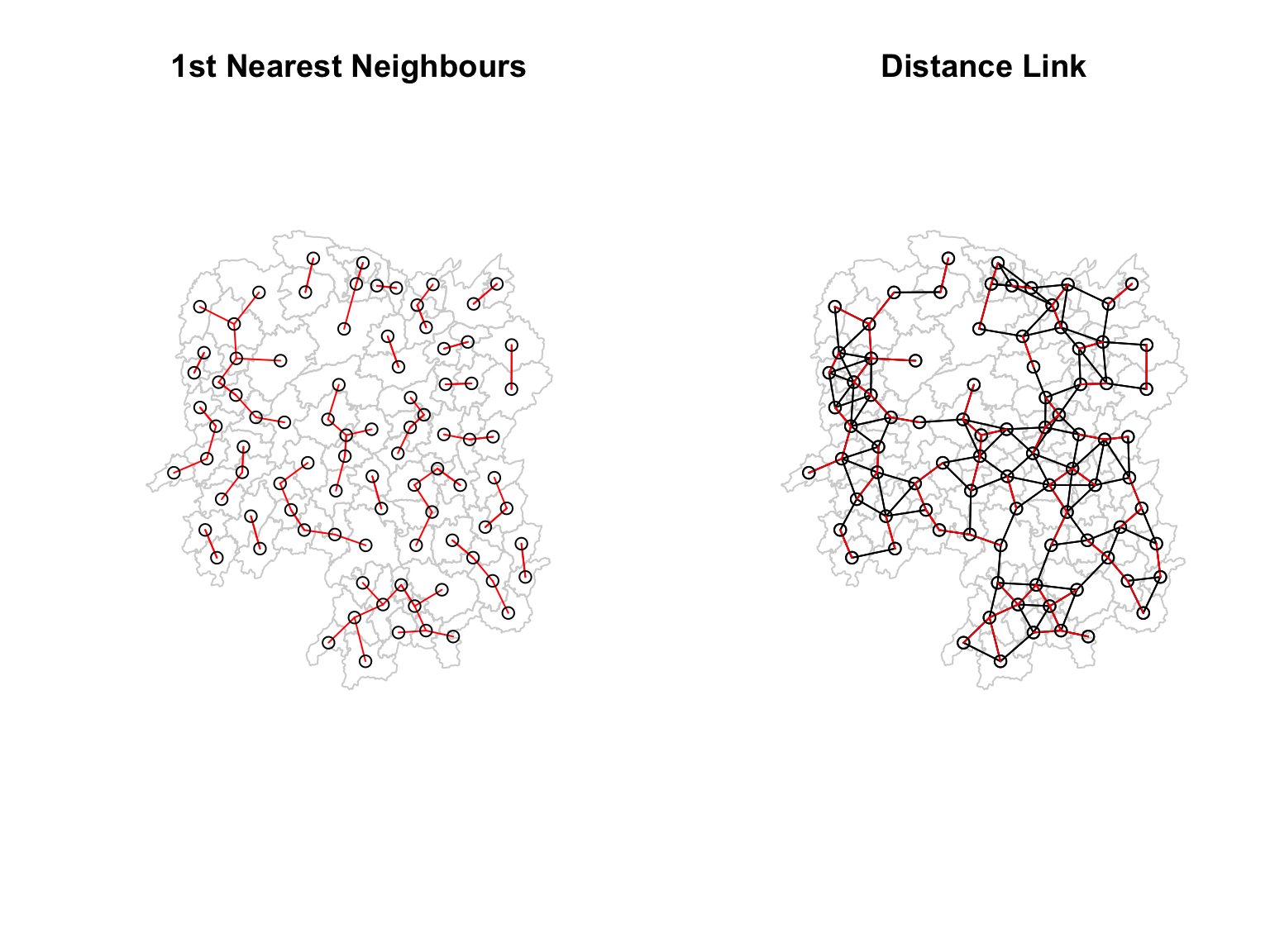
On the left plot, the red lines show the links of 1st nearest neighbours.

On the right plot, the red lines show the links of 1st nearest neighbours and the black lines show the links of neighbours within the cut-off distance of 62km.

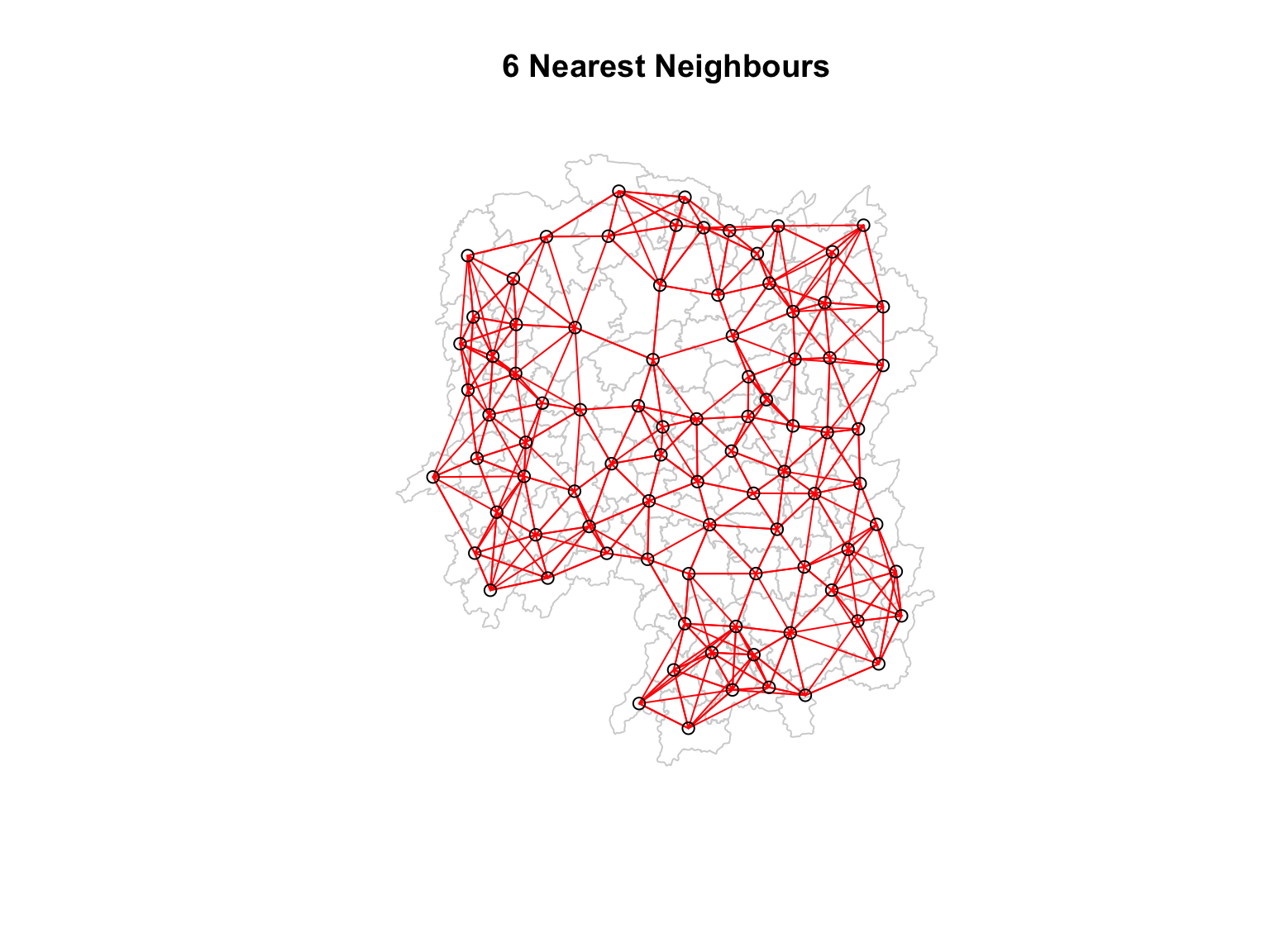
10.4 Computing Adaptive Distance Weight Matrix

A fixed distance weight matrix typically shows that densely populated areas (like urban regions) have more neighbors, while sparsely populated areas (such as rural counties) have fewer neighbors. When there are many neighbors, the relationships between them are spread across a larger number of connections, creating a smoother effect.

To control the number of neighbours, we can set the k value.

knn6 <- knn2nb(knearneigh(coords, k=6))
knn6

Neighbour list object:
Number of regions: 88
Number of nonzero links: 528
Percentage nonzero weights: 6.818182
Average number of links: 6
Non-symmetric neighbours list

Each county has exactly 6 neighbours.

str(knn6)

10.4.1 Computing Adaptive Distance Weight Matrix

plot(hunan$geometry, border="lightgrey", main="6 Nearest Neighbours")
plot(knn6, coords, add = TRUE, col = "red")

11 Weights based on Inversed Distance Weight (IDW) Method

In this section, you will learn how to derive a spatial weight matrix based on Inversed Distance Weights method.

Note

In order to conform to Tobler’s first law of geography, a distance decay effect must be respected.

The inverse distance weight method assigns weights to neighbors based on their distance: closer neighbors get higher weights, and further ones get lower weights.

It works by taking the distance between two locations and calculating the weight as 1 divided by that distance.

For more info, see Spatial Weights as Distance Functions.

dist <- nbdists(wm_q, 
                coords, 
                longlat = TRUE)
# apply 1/x on every element on list objects
ids <- lapply(dist, function(x) 1/(x))

12 Row-standardised Weights Matrix

Next, we need to assign weights to each neighboring polygon. In this case, we’ll use equal weights (style=“W”), where each neighboring polygon gets a weight of 1/(number of neighbors). This means we take the value for each neighbor and divide it by the total number of neighbors, then sum these weighted values to calculate a summary measure, such as weighted income.

While this equal weighting approach is straightforward and easy to understand, it has a limitation: polygons on the edges of the study area have fewer neighbors, which can lead to over- or underestimation of the actual spatial relationships (spatial autocorrelation) in the data.

Tip

For simplicity, we use the style=“W” option in this example, but keep in mind that other, potentially more accurate methods are available, such as style=“B”.

# note we are using queen's method here
rswm_q <- nb2listw(wm_q, style="W", zero.policy = TRUE)
rswm_q

Characteristics of weights list object:
Neighbour list object:
Number of regions: 88
Number of nonzero links: 448
Percentage nonzero weights: 5.785124
Average number of links: 5.090909

Weights style: W
Weights constants summary:
   n   nn S0       S1       S2
W 88 7744 88 37.86334 365.9147

Tip

The zero.policy=TRUE option allows for lists of non-neighbors. This should be used with caution since the user may not be aware of missing neighbors in their dataset however, a zero.policy of FALSE would return an error.

To see the weight of the 85th polygon’s 11 neighbors type:

rswm_q$weights[85]

[[1]]
 [1] 0.09090909 0.09090909 0.09090909 0.09090909 0.09090909 0.09090909
 [7] 0.09090909 0.09090909 0.09090909 0.09090909 0.09090909

Each neighbor is assigned a 0.0909 of the total weight. This means that when R computes the average neighboring income values, each neighbor’s income will be multiplied by 0.0909 before being tallied.

Using the same method, we can also derive a row standardised distance weight matrix by using the code block below.

rswm_ids <- nb2listw(wm_q, glist=ids, style="B", zero.policy=TRUE)
rswm_ids

Characteristics of weights list object:
Neighbour list object:
Number of regions: 88
Number of nonzero links: 448
Percentage nonzero weights: 5.785124
Average number of links: 5.090909

Weights style: B
Weights constants summary:
   n   nn       S0        S1     S2
B 88 7744 8.786867 0.3776535 3.8137

rswm_ids$weights[85]

[[1]]
 [1] 0.011451133 0.017193502 0.013957649 0.016183544 0.009810297 0.010656545
 [7] 0.013416965 0.009903702 0.014199260 0.008217581 0.011407794

Notice that the output has different weight of each neighbour. We can use summary report to observe the differences.

summary(unlist(rswm_q$weights))

   Min. 1st Qu.  Median    Mean 3rd Qu.    Max.
0.09091 0.14286 0.20000 0.19643 0.20000 1.00000

cat("\n-----------------------------\n")


-----------------------------

summary(unlist(rswm_ids$weights))

    Min.  1st Qu.   Median     Mean  3rd Qu.     Max.
0.008218 0.015088 0.018739 0.019614 0.022823 0.040338

13 Application of Spatial Weight Matrix

In this section, we will create 4 different spatial lagged variables:

spatial lag with row-standardized weights,
spatial lag as a sum of neighbouring values,
spatial window average, and
spatial window sum.

13.1 Spatial Lag with Row-standardized Weights

We’ll compute the average neighbor GDPPC value for each polygon. These values are often referred to as spatially lagged values.

GDPPC.lag <- lag.listw(rswm_q, hunan$GDPPC)
GDPPC.lag

 [1] 24847.20 22724.80 24143.25 27737.50 27270.25 21248.80 43747.00 33582.71
 [9] 45651.17 32027.62 32671.00 20810.00 25711.50 30672.33 33457.75 31689.20
[17] 20269.00 23901.60 25126.17 21903.43 22718.60 25918.80 20307.00 20023.80
[25] 16576.80 18667.00 14394.67 19848.80 15516.33 20518.00 17572.00 15200.12
[33] 18413.80 14419.33 24094.50 22019.83 12923.50 14756.00 13869.80 12296.67
[41] 15775.17 14382.86 11566.33 13199.50 23412.00 39541.00 36186.60 16559.60
[49] 20772.50 19471.20 19827.33 15466.80 12925.67 18577.17 14943.00 24913.00
[57] 25093.00 24428.80 17003.00 21143.75 20435.00 17131.33 24569.75 23835.50
[65] 26360.00 47383.40 55157.75 37058.00 21546.67 23348.67 42323.67 28938.60
[73] 25880.80 47345.67 18711.33 29087.29 20748.29 35933.71 15439.71 29787.50
[81] 18145.00 21617.00 29203.89 41363.67 22259.09 44939.56 16902.00 16930.00

In the previous section, we retrieved the GDPPC of these 11 counties by using the code block below.

nb1 <- wm_q[[85]]
nb1 <- hunan$GDPPC[nb1]
nb1

 [1] 23667 20981 34592 25554 27137 24194 14567 21311 18714 14624 19509

Question: Can you see the meaning of Spatial lag with row-standardized weights now? Spatial lag represents the average or sum of a variable (GDPPC) for a region’s neighbors. In this context, the spatial lag for a region gives an idea of how that region’s GDPPC relates to the GDPPC of its neighboring regions.

With row-standardized weights (style=“W”), each neighboring region is assigned an equal weight of 1/(number of neighbors). This ensures that the weights for all neighbors of a region sum to 1.

We can append the spatially lag GDPPC values onto hunan sf data frame by using the code block below:

lag.list <- list(hunan$NAME_3, lag.listw(rswm_q, hunan$GDPPC))
lag.res <- as.data.frame(lag.list)
colnames(lag.res) <- c("NAME_3", "lag GDPPC")
hunan <- left_join(hunan,lag.res)

The following table shows the average neighboring income values (stored in the Inc.lag object) for each county.

head(hunan)

Simple feature collection with 6 features and 7 fields
Geometry type: POLYGON
Dimension:     XY
Bounding box:  xmin: 110.4922 ymin: 28.61762 xmax: 112.3013 ymax: 30.12812
Geodetic CRS:  WGS 84
   NAME_2  ID_3  NAME_3   ENGTYPE_3  County GDPPC lag GDPPC
1 Changde 21098 Anxiang      County Anxiang 23667  24847.20
2 Changde 21100 Hanshou      County Hanshou 20981  22724.80
3 Changde 21101  Jinshi County City  Jinshi 34592  24143.25
4 Changde 21102      Li      County      Li 24473  27737.50
5 Changde 21103   Linli      County   Linli 25554  27270.25
6 Changde 21104  Shimen      County  Shimen 27137  21248.80
                        geometry
1 POLYGON ((112.0625 29.75523...
2 POLYGON ((112.2288 29.11684...
3 POLYGON ((111.8927 29.6013,...
4 POLYGON ((111.3731 29.94649...
5 POLYGON ((111.6324 29.76288...
6 POLYGON ((110.8825 30.11675...

Next, we will plot both the GDPPC and spatial lag GDPPC for comparison using the code block below.

gdppc <- qtm(hunan, "GDPPC")
lag_gdppc <- qtm(hunan, "lag GDPPC")
tmap_arrange(gdppc, lag_gdppc, asp=1, ncol=2)

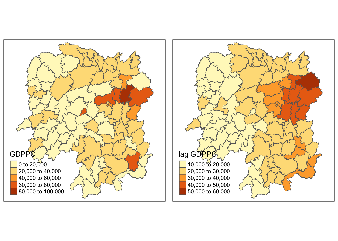
Recall that in our previous observation, we made the statement that Changsha has the highest GDP per capital values in the Hunan region.

Using spatial lag values, we can observe that Yueyang has the highest spatial lag GDP per capita, meaning its neighbors (on average) have the highest GDP per capita.

13.2 Spatial Lag as a Sum of Neighboring Values

To calculate spatial lag as the sum of neighboring values, we can assign binary weights (where each neighbor gets a weight of 1).

To do this, we go back to our list of neighbors and use a function to assign these binary weights. We then use the glist argument in the nb2listw function to set these weights explicitly.

We start by using lapply to assign a weight of 1 to each neighbor. lapply is a function we have been using to work with the neighbors list in previous notebooks; it applies a specified function to each value in the neighbors list.

# Create binary weights for each neighbor
# uses lapply to go through each element of the neighbors list (wm_q).
# The function '0 * x + 1' assigns a weight of 1 to each neighbor.
b_weights <- lapply(wm_q, function(x) 0*x + 1)

# Convert the neighbor list to a spatial weights list object
# 'nb2listw' converts the neighbors list (wm_q) into a weights list.
# 'glist = b_weights' explicitly sets the weights to the binary weights created above.
# 'style = "B"' specifies binary weighting style, where each neighbor has equal weight (1).
b_weights2 <- nb2listw(wm_q, 
                       glist = b_weights, 
                       style = "B")
b_weights2

Characteristics of weights list object:
Neighbour list object:
Number of regions: 88
Number of nonzero links: 448
Percentage nonzero weights: 5.785124
Average number of links: 5.090909

Weights style: B
Weights constants summary:
   n   nn  S0  S1    S2
B 88 7744 448 896 10224

With the proper weights assigned, we can use lag.listw to compute a lag variable from our weight and GDPPC.

lag_sum <- list(hunan$NAME_3, lag.listw(b_weights2, hunan$GDPPC))
lag.res <- as.data.frame(lag_sum)
colnames(lag.res) <- c("NAME_3", "lag_sum GDPPC")
lag_sum

[[1]]
 [1] "Anxiang"       "Hanshou"       "Jinshi"        "Li"
 [5] "Linli"         "Shimen"        "Liuyang"       "Ningxiang"
 [9] "Wangcheng"     "Anren"         "Guidong"       "Jiahe"
[13] "Linwu"         "Rucheng"       "Yizhang"       "Yongxing"
[17] "Zixing"        "Changning"     "Hengdong"      "Hengnan"
[21] "Hengshan"      "Leiyang"       "Qidong"        "Chenxi"
[25] "Zhongfang"     "Huitong"       "Jingzhou"      "Mayang"
[29] "Tongdao"       "Xinhuang"      "Xupu"          "Yuanling"
[33] "Zhijiang"      "Lengshuijiang" "Shuangfeng"    "Xinhua"
[37] "Chengbu"       "Dongan"        "Dongkou"       "Longhui"
[41] "Shaodong"      "Suining"       "Wugang"        "Xinning"
[45] "Xinshao"       "Shaoshan"      "Xiangxiang"    "Baojing"
[49] "Fenghuang"     "Guzhang"       "Huayuan"       "Jishou"
[53] "Longshan"      "Luxi"          "Yongshun"      "Anhua"
[57] "Nan"           "Yuanjiang"     "Jianghua"      "Lanshan"
[61] "Ningyuan"      "Shuangpai"     "Xintian"       "Huarong"
[65] "Linxiang"      "Miluo"         "Pingjiang"     "Xiangyin"
[69] "Cili"          "Chaling"       "Liling"        "Yanling"
[73] "You"           "Zhuzhou"       "Sangzhi"       "Yueyang"
[77] "Qiyang"        "Taojiang"      "Shaoyang"      "Lianyuan"
[81] "Hongjiang"     "Hengyang"      "Guiyang"       "Changsha"
[85] "Taoyuan"       "Xiangtan"      "Dao"           "Jiangyong"

[[2]]
 [1] 124236 113624  96573 110950 109081 106244 174988 235079 273907 256221
[11]  98013 104050 102846  92017 133831 158446 141883 119508 150757 153324
[21] 113593 129594 142149 100119  82884  74668  43184  99244  46549  20518
[31] 140576 121601  92069  43258 144567 132119  51694  59024  69349  73780
[41]  94651 100680  69398  52798 140472 118623 180933  82798  83090  97356
[51]  59482  77334  38777 111463  74715 174391 150558 122144  68012  84575
[61] 143045  51394  98279  47671  26360 236917 220631 185290  64640  70046
[71] 126971 144693 129404 284074 112268 203611 145238 251536 108078 238300
[81] 108870 108085 262835 248182 244850 404456  67608  33860

Question: Can you understand the meaning of Spatial lag as a sum of neighboring values now?

By assigning binary weights (where each neighbor is given a weight of 1), we calculate the spatial lag by summing the values of this variable for all neighbors. This means that the spatial lag reflects the combined influence or total value contributed by the neighboring regions, providing an idea of the overall regional context or neighborhood effect around a specific area.

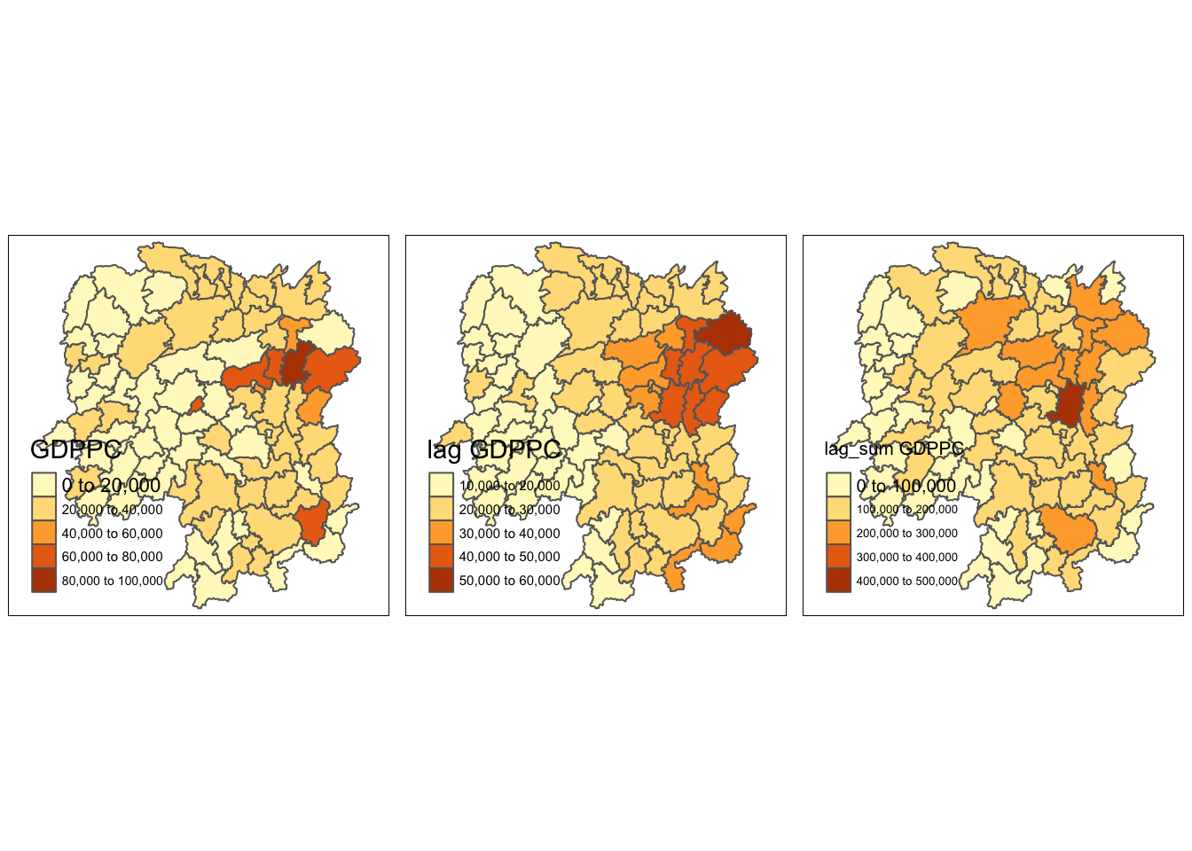
Next, we will append the lag_sum GDPPC field into hunan sf data frame by using the code block below.

hunan <- left_join(hunan, lag.res)

Now, we can plot the GDPPC, Spatial Lag GDPPC, Spatial Lag Sum GDPPC for comparison using the code block below.

gdppc <- qtm(hunan, "GDPPC")
lag_gdppc <- qtm(hunan, "lag GDPPC")
lag_sum_gdppc <- qtm(hunan, "lag_sum GDPPC")
tmap_arrange(gdppc, lag_gdppc, lag_sum_gdppc, asp=1, ncol=3)

13.3 Spatial Window Average

The spatial window average uses row-standardized weights and includes the diagonal element. To do this in R, we need to go back to the neighbors structure and add the diagonal element before assigning weights.

To add the diagonal element to the neighbour list, we just need to use include.self() from spdep.

wm_qs <- include.self(wm_q)

Let us take a good look at the neighbour list of area 85 by using the code block below.

wm_qs[[85]]

 [1]  1  2  3  5  6 32 56 57 69 75 78 85

Notice that now region 85 has 12 neighbours instead of 11.

Now we obtain weights with nb2listw().

wm_qs <- nb2listw(wm_qs)
wm_qs

Characteristics of weights list object:
Neighbour list object:
Number of regions: 88
Number of nonzero links: 536
Percentage nonzero weights: 6.921488
Average number of links: 6.090909

Weights style: W
Weights constants summary:
   n   nn S0       S1       S2
W 88 7744 88 30.90265 357.5308

Again, we use nb2listw() and glist() to explicitly assign weight values.

Lastly, we just need to create the lag variable from our weight structure and GDPPC variable.

lag_w_avg_gpdpc <- lag.listw(wm_qs, 
                             hunan$GDPPC)
lag_w_avg_gpdpc

 [1] 24650.50 22434.17 26233.00 27084.60 26927.00 22230.17 47621.20 37160.12
 [9] 49224.71 29886.89 26627.50 22690.17 25366.40 25825.75 30329.00 32682.83
[17] 25948.62 23987.67 25463.14 21904.38 23127.50 25949.83 20018.75 19524.17
[25] 18955.00 17800.40 15883.00 18831.33 14832.50 17965.00 17159.89 16199.44
[33] 18764.50 26878.75 23188.86 20788.14 12365.20 15985.00 13764.83 11907.43
[41] 17128.14 14593.62 11644.29 12706.00 21712.29 43548.25 35049.00 16226.83
[49] 19294.40 18156.00 19954.75 18145.17 12132.75 18419.29 14050.83 23619.75
[57] 24552.71 24733.67 16762.60 20932.60 19467.75 18334.00 22541.00 26028.00
[65] 29128.50 46569.00 47576.60 36545.50 20838.50 22531.00 42115.50 27619.00
[73] 27611.33 44523.29 18127.43 28746.38 20734.50 33880.62 14716.38 28516.22
[81] 18086.14 21244.50 29568.80 48119.71 22310.75 43151.60 17133.40 17009.33

Next, we will convert the lag variable listw object into a data.frame by using as.data.frame().

lag.list.wm_qs <- list(hunan$NAME_3, lag.listw(wm_qs, hunan$GDPPC))
lag_wm_qs.res <- as.data.frame(lag.list.wm_qs)
colnames(lag_wm_qs.res) <- c("NAME_3", "lag_window_avg GDPPC")

Note

The third command line on the code chunk above renames the field names of lag_wm_q1.res object into NAME_3 and lag_window_avg GDPPC respectively.

Next, the code chunk below will be used to append lag_window_avg GDPPC values onto hunan sf data.frame by using left_join() of dplyr package.

hunan <- left_join(hunan, lag_wm_qs.res)

To compare the values of lag GDPPC and Spatial window average, kable() of Knitr package is used to prepare a table using the code chunk below.

hunan %>%
  select("County", 
         "lag GDPPC", 
         "lag_window_avg GDPPC") %>%
  kable()

County	lag GDPPC	lag_window_avg GDPPC	geometry
Anxiang	24847.20	24650.50	POLYGON ((112.0625 29.75523…
Hanshou	22724.80	22434.17	POLYGON ((112.2288 29.11684…
Jinshi	24143.25	26233.00	POLYGON ((111.8927 29.6013,…
Li	27737.50	27084.60	POLYGON ((111.3731 29.94649…
Linli	27270.25	26927.00	POLYGON ((111.6324 29.76288…
Shimen	21248.80	22230.17	POLYGON ((110.8825 30.11675…
Liuyang	43747.00	47621.20	POLYGON ((113.9905 28.5682,…
Ningxiang	33582.71	37160.12	POLYGON ((112.7181 28.38299…
Wangcheng	45651.17	49224.71	POLYGON ((112.7914 28.52688…
Anren	32027.62	29886.89	POLYGON ((113.1757 26.82734…
Guidong	32671.00	26627.50	POLYGON ((114.1799 26.20117…
Jiahe	20810.00	22690.17	POLYGON ((112.4425 25.74358…
Linwu	25711.50	25366.40	POLYGON ((112.5914 25.55143…
Rucheng	30672.33	25825.75	POLYGON ((113.6759 25.87578…
Yizhang	33457.75	30329.00	POLYGON ((113.2621 25.68394…
Yongxing	31689.20	32682.83	POLYGON ((113.3169 26.41843…
Zixing	20269.00	25948.62	POLYGON ((113.7311 26.16259…
Changning	23901.60	23987.67	POLYGON ((112.6144 26.60198…
Hengdong	25126.17	25463.14	POLYGON ((113.1056 27.21007…
Hengnan	21903.43	21904.38	POLYGON ((112.7599 26.98149…
Hengshan	22718.60	23127.50	POLYGON ((112.607 27.4689, …
Leiyang	25918.80	25949.83	POLYGON ((112.9996 26.69276…
Qidong	20307.00	20018.75	POLYGON ((111.7818 27.0383,…
Chenxi	20023.80	19524.17	POLYGON ((110.2624 28.21778…
Zhongfang	16576.80	18955.00	POLYGON ((109.9431 27.72858…
Huitong	18667.00	17800.40	POLYGON ((109.9419 27.10512…
Jingzhou	14394.67	15883.00	POLYGON ((109.8186 26.75842…
Mayang	19848.80	18831.33	POLYGON ((109.795 27.98008,…
Tongdao	15516.33	14832.50	POLYGON ((109.9294 26.46561…
Xinhuang	20518.00	17965.00	POLYGON ((109.227 27.43733,…
Xupu	17572.00	17159.89	POLYGON ((110.7189 28.30485…
Yuanling	15200.12	16199.44	POLYGON ((110.9652 28.99895…
Zhijiang	18413.80	18764.50	POLYGON ((109.8818 27.60661…
Lengshuijiang	14419.33	26878.75	POLYGON ((111.5307 27.81472…
Shuangfeng	24094.50	23188.86	POLYGON ((112.263 27.70421,…
Xinhua	22019.83	20788.14	POLYGON ((111.3345 28.19642…
Chengbu	12923.50	12365.20	POLYGON ((110.4455 26.69317…
Dongan	14756.00	15985.00	POLYGON ((111.4531 26.86812…
Dongkou	13869.80	13764.83	POLYGON ((110.6622 27.37305…
Longhui	12296.67	11907.43	POLYGON ((110.985 27.65983,…
Shaodong	15775.17	17128.14	POLYGON ((111.9054 27.40254…
Suining	14382.86	14593.62	POLYGON ((110.389 27.10006,…
Wugang	11566.33	11644.29	POLYGON ((110.9878 27.03345…
Xinning	13199.50	12706.00	POLYGON ((111.0736 26.84627…
Xinshao	23412.00	21712.29	POLYGON ((111.6013 27.58275…
Shaoshan	39541.00	43548.25	POLYGON ((112.5391 27.97742…
Xiangxiang	36186.60	35049.00	POLYGON ((112.4549 28.05783…
Baojing	16559.60	16226.83	POLYGON ((109.7015 28.82844…
Fenghuang	20772.50	19294.40	POLYGON ((109.5239 28.19206…
Guzhang	19471.20	18156.00	POLYGON ((109.8968 28.74034…
Huayuan	19827.33	19954.75	POLYGON ((109.5647 28.61712…
Jishou	15466.80	18145.17	POLYGON ((109.8375 28.4696,…
Longshan	12925.67	12132.75	POLYGON ((109.6337 29.62521…
Luxi	18577.17	18419.29	POLYGON ((110.1067 28.41835…
Yongshun	14943.00	14050.83	POLYGON ((110.0003 29.29499…
Anhua	24913.00	23619.75	POLYGON ((111.6034 28.63716…
Nan	25093.00	24552.71	POLYGON ((112.3232 29.46074…
Yuanjiang	24428.80	24733.67	POLYGON ((112.4391 29.1791,…
Jianghua	17003.00	16762.60	POLYGON ((111.6461 25.29661…
Lanshan	21143.75	20932.60	POLYGON ((112.2286 25.61123…
Ningyuan	20435.00	19467.75	POLYGON ((112.0715 26.09892…
Shuangpai	17131.33	18334.00	POLYGON ((111.8864 26.11957…
Xintian	24569.75	22541.00	POLYGON ((112.2578 26.0796,…
Huarong	23835.50	26028.00	POLYGON ((112.9242 29.69134…
Linxiang	26360.00	29128.50	POLYGON ((113.5502 29.67418…
Miluo	47383.40	46569.00	POLYGON ((112.9902 29.02139…
Pingjiang	55157.75	47576.60	POLYGON ((113.8436 29.06152…
Xiangyin	37058.00	36545.50	POLYGON ((112.9173 28.98264…
Cili	21546.67	20838.50	POLYGON ((110.8822 29.69017…
Chaling	23348.67	22531.00	POLYGON ((113.7666 27.10573…
Liling	42323.67	42115.50	POLYGON ((113.5673 27.94346…
Yanling	28938.60	27619.00	POLYGON ((113.9292 26.6154,…
You	25880.80	27611.33	POLYGON ((113.5879 27.41324…
Zhuzhou	47345.67	44523.29	POLYGON ((113.2493 28.02411…
Sangzhi	18711.33	18127.43	POLYGON ((110.556 29.40543,…
Yueyang	29087.29	28746.38	POLYGON ((113.343 29.61064,…
Qiyang	20748.29	20734.50	POLYGON ((111.5563 26.81318…
Taojiang	35933.71	33880.62	POLYGON ((112.0508 28.67265…
Shaoyang	15439.71	14716.38	POLYGON ((111.5013 27.30207…
Lianyuan	29787.50	28516.22	POLYGON ((111.6789 28.02946…
Hongjiang	18145.00	18086.14	POLYGON ((110.1441 27.47513…
Hengyang	21617.00	21244.50	POLYGON ((112.7144 26.98613…
Guiyang	29203.89	29568.80	POLYGON ((113.0811 26.04963…
Changsha	41363.67	48119.71	POLYGON ((112.9421 28.03722…
Taoyuan	22259.09	22310.75	POLYGON ((112.0612 29.32855…
Xiangtan	44939.56	43151.60	POLYGON ((113.0426 27.8942,…
Dao	16902.00	17133.40	POLYGON ((111.498 25.81679,…
Jiangyong	16930.00	17009.33	POLYGON ((111.3659 25.39472…

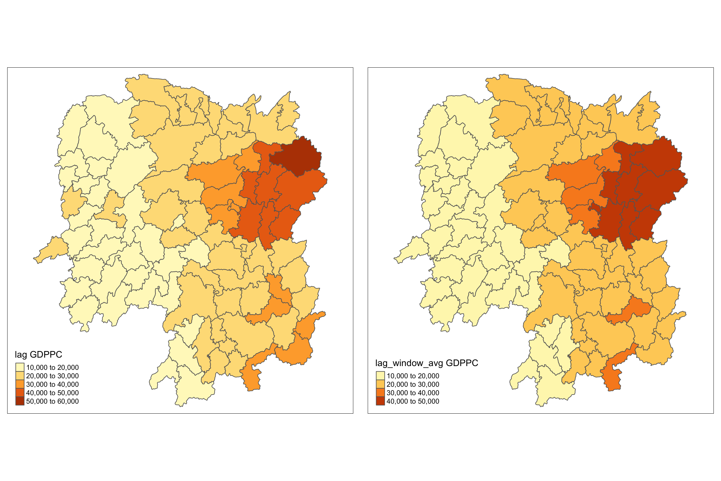
Lastly, qtm() of tmap package is used to plot the lag_gdppc and w_ave_gdppc maps next to each other for quick comparison.

w_avg_gdppc <- qtm(hunan, "lag_window_avg GDPPC")
tmap_arrange(lag_gdppc, w_avg_gdppc, asp=1, ncol=2)

Tip

For more effective comparison, it is advisable to use the core tmap mapping functions.

13.4 Spatial Window Sum

The spatial window sum is the counter part of the window average, but without using row-standardized weights.

To add the diagonal element to the neighbour list, we just need to use include.self() from spdep.

wm_qs <- include.self(wm_q)
wm_qs

Neighbour list object:
Number of regions: 88
Number of nonzero links: 536
Percentage nonzero weights: 6.921488
Average number of links: 6.090909

Next, we will assign binary weights to the neighbour structure that includes the diagonal element.

b_weights <- lapply(wm_qs, function(x) 0*x + 1)
b_weights[1]

[[1]]
[1] 1 1 1 1 1 1

Notice that now region 85 has 12 neighbours instead of 11.

Again, we use nb2listw() and glist() to explicitly assign weight values.

b_weights2 <- nb2listw(wm_qs, 
                       glist = b_weights, 
                       style = "B")
b_weights2

Characteristics of weights list object:
Neighbour list object:
Number of regions: 88
Number of nonzero links: 536
Percentage nonzero weights: 6.921488
Average number of links: 6.090909

Weights style: B
Weights constants summary:
   n   nn  S0   S1    S2
B 88 7744 536 1072 14160

With our new weight structure, we can compute the lag variable with lag.listw().

w_sum_gdppc <- list(hunan$NAME_3, lag.listw(b_weights2, hunan$GDPPC))
w_sum_gdppc

[[1]]
 [1] "Anxiang"       "Hanshou"       "Jinshi"        "Li"
 [5] "Linli"         "Shimen"        "Liuyang"       "Ningxiang"
 [9] "Wangcheng"     "Anren"         "Guidong"       "Jiahe"
[13] "Linwu"         "Rucheng"       "Yizhang"       "Yongxing"
[17] "Zixing"        "Changning"     "Hengdong"      "Hengnan"
[21] "Hengshan"      "Leiyang"       "Qidong"        "Chenxi"
[25] "Zhongfang"     "Huitong"       "Jingzhou"      "Mayang"
[29] "Tongdao"       "Xinhuang"      "Xupu"          "Yuanling"
[33] "Zhijiang"      "Lengshuijiang" "Shuangfeng"    "Xinhua"
[37] "Chengbu"       "Dongan"        "Dongkou"       "Longhui"
[41] "Shaodong"      "Suining"       "Wugang"        "Xinning"
[45] "Xinshao"       "Shaoshan"      "Xiangxiang"    "Baojing"
[49] "Fenghuang"     "Guzhang"       "Huayuan"       "Jishou"
[53] "Longshan"      "Luxi"          "Yongshun"      "Anhua"
[57] "Nan"           "Yuanjiang"     "Jianghua"      "Lanshan"
[61] "Ningyuan"      "Shuangpai"     "Xintian"       "Huarong"
[65] "Linxiang"      "Miluo"         "Pingjiang"     "Xiangyin"
[69] "Cili"          "Chaling"       "Liling"        "Yanling"
[73] "You"           "Zhuzhou"       "Sangzhi"       "Yueyang"
[77] "Qiyang"        "Taojiang"      "Shaoyang"      "Lianyuan"
[81] "Hongjiang"     "Hengyang"      "Guiyang"       "Changsha"
[85] "Taoyuan"       "Xiangtan"      "Dao"           "Jiangyong"

[[2]]
 [1] 147903 134605 131165 135423 134635 133381 238106 297281 344573 268982
[11] 106510 136141 126832 103303 151645 196097 207589 143926 178242 175235
[21] 138765 155699 160150 117145 113730  89002  63532 112988  59330  35930
[31] 154439 145795 112587 107515 162322 145517  61826  79925  82589  83352
[41] 119897 116749  81510  63530 151986 174193 210294  97361  96472 108936
[51]  79819 108871  48531 128935  84305 188958 171869 148402  83813 104663
[61] 155742  73336 112705  78084  58257 279414 237883 219273  83354  90124
[71] 168462 165714 165668 311663 126892 229971 165876 271045 117731 256646
[81] 126603 127467 295688 336838 267729 431516  85667  51028

Next, we will convert the lag variable listw object into a data.frame by using as.data.frame().

w_sum_gdppc.res <- as.data.frame(w_sum_gdppc)
colnames(w_sum_gdppc.res) <- c("NAME_3", "w_sum GDPPC")

Note: The second command line on the code chunk above renames the field names of w_sum_gdppc.res object into NAME_3 and w_sum GDPPC respectively.

Next, the code chunk below will be used to append w_sum GDPPC values onto hunan sf data.frame by using left_join() of dplyr package.

hunan <- left_join(hunan, w_sum_gdppc.res)

To compare the values of lag GDPPC and Spatial window average, kable() of Knitr package is used to prepare a table using the code chunk below.

hunan %>%
  select("County", "lag_sum GDPPC", "w_sum GDPPC") %>%
  kable()

County	lag_sum GDPPC	w_sum GDPPC	geometry
Anxiang	124236	147903	POLYGON ((112.0625 29.75523…
Hanshou	113624	134605	POLYGON ((112.2288 29.11684…
Jinshi	96573	131165	POLYGON ((111.8927 29.6013,…
Li	110950	135423	POLYGON ((111.3731 29.94649…
Linli	109081	134635	POLYGON ((111.6324 29.76288…
Shimen	106244	133381	POLYGON ((110.8825 30.11675…
Liuyang	174988	238106	POLYGON ((113.9905 28.5682,…
Ningxiang	235079	297281	POLYGON ((112.7181 28.38299…
Wangcheng	273907	344573	POLYGON ((112.7914 28.52688…
Anren	256221	268982	POLYGON ((113.1757 26.82734…
Guidong	98013	106510	POLYGON ((114.1799 26.20117…
Jiahe	104050	136141	POLYGON ((112.4425 25.74358…
Linwu	102846	126832	POLYGON ((112.5914 25.55143…
Rucheng	92017	103303	POLYGON ((113.6759 25.87578…
Yizhang	133831	151645	POLYGON ((113.2621 25.68394…
Yongxing	158446	196097	POLYGON ((113.3169 26.41843…
Zixing	141883	207589	POLYGON ((113.7311 26.16259…
Changning	119508	143926	POLYGON ((112.6144 26.60198…
Hengdong	150757	178242	POLYGON ((113.1056 27.21007…
Hengnan	153324	175235	POLYGON ((112.7599 26.98149…
Hengshan	113593	138765	POLYGON ((112.607 27.4689, …
Leiyang	129594	155699	POLYGON ((112.9996 26.69276…
Qidong	142149	160150	POLYGON ((111.7818 27.0383,…
Chenxi	100119	117145	POLYGON ((110.2624 28.21778…
Zhongfang	82884	113730	POLYGON ((109.9431 27.72858…
Huitong	74668	89002	POLYGON ((109.9419 27.10512…
Jingzhou	43184	63532	POLYGON ((109.8186 26.75842…
Mayang	99244	112988	POLYGON ((109.795 27.98008,…
Tongdao	46549	59330	POLYGON ((109.9294 26.46561…
Xinhuang	20518	35930	POLYGON ((109.227 27.43733,…
Xupu	140576	154439	POLYGON ((110.7189 28.30485…
Yuanling	121601	145795	POLYGON ((110.9652 28.99895…
Zhijiang	92069	112587	POLYGON ((109.8818 27.60661…
Lengshuijiang	43258	107515	POLYGON ((111.5307 27.81472…
Shuangfeng	144567	162322	POLYGON ((112.263 27.70421,…
Xinhua	132119	145517	POLYGON ((111.3345 28.19642…
Chengbu	51694	61826	POLYGON ((110.4455 26.69317…
Dongan	59024	79925	POLYGON ((111.4531 26.86812…
Dongkou	69349	82589	POLYGON ((110.6622 27.37305…
Longhui	73780	83352	POLYGON ((110.985 27.65983,…
Shaodong	94651	119897	POLYGON ((111.9054 27.40254…
Suining	100680	116749	POLYGON ((110.389 27.10006,…
Wugang	69398	81510	POLYGON ((110.9878 27.03345…
Xinning	52798	63530	POLYGON ((111.0736 26.84627…
Xinshao	140472	151986	POLYGON ((111.6013 27.58275…
Shaoshan	118623	174193	POLYGON ((112.5391 27.97742…
Xiangxiang	180933	210294	POLYGON ((112.4549 28.05783…
Baojing	82798	97361	POLYGON ((109.7015 28.82844…
Fenghuang	83090	96472	POLYGON ((109.5239 28.19206…
Guzhang	97356	108936	POLYGON ((109.8968 28.74034…
Huayuan	59482	79819	POLYGON ((109.5647 28.61712…
Jishou	77334	108871	POLYGON ((109.8375 28.4696,…
Longshan	38777	48531	POLYGON ((109.6337 29.62521…
Luxi	111463	128935	POLYGON ((110.1067 28.41835…
Yongshun	74715	84305	POLYGON ((110.0003 29.29499…
Anhua	174391	188958	POLYGON ((111.6034 28.63716…
Nan	150558	171869	POLYGON ((112.3232 29.46074…
Yuanjiang	122144	148402	POLYGON ((112.4391 29.1791,…
Jianghua	68012	83813	POLYGON ((111.6461 25.29661…
Lanshan	84575	104663	POLYGON ((112.2286 25.61123…
Ningyuan	143045	155742	POLYGON ((112.0715 26.09892…
Shuangpai	51394	73336	POLYGON ((111.8864 26.11957…
Xintian	98279	112705	POLYGON ((112.2578 26.0796,…
Huarong	47671	78084	POLYGON ((112.9242 29.69134…
Linxiang	26360	58257	POLYGON ((113.5502 29.67418…
Miluo	236917	279414	POLYGON ((112.9902 29.02139…
Pingjiang	220631	237883	POLYGON ((113.8436 29.06152…
Xiangyin	185290	219273	POLYGON ((112.9173 28.98264…
Cili	64640	83354	POLYGON ((110.8822 29.69017…
Chaling	70046	90124	POLYGON ((113.7666 27.10573…
Liling	126971	168462	POLYGON ((113.5673 27.94346…
Yanling	144693	165714	POLYGON ((113.9292 26.6154,…
You	129404	165668	POLYGON ((113.5879 27.41324…
Zhuzhou	284074	311663	POLYGON ((113.2493 28.02411…
Sangzhi	112268	126892	POLYGON ((110.556 29.40543,…
Yueyang	203611	229971	POLYGON ((113.343 29.61064,…
Qiyang	145238	165876	POLYGON ((111.5563 26.81318…
Taojiang	251536	271045	POLYGON ((112.0508 28.67265…
Shaoyang	108078	117731	POLYGON ((111.5013 27.30207…
Lianyuan	238300	256646	POLYGON ((111.6789 28.02946…
Hongjiang	108870	126603	POLYGON ((110.1441 27.47513…
Hengyang	108085	127467	POLYGON ((112.7144 26.98613…
Guiyang	262835	295688	POLYGON ((113.0811 26.04963…
Changsha	248182	336838	POLYGON ((112.9421 28.03722…
Taoyuan	244850	267729	POLYGON ((112.0612 29.32855…
Xiangtan	404456	431516	POLYGON ((113.0426 27.8942,…
Dao	67608	85667	POLYGON ((111.498 25.81679,…
Jiangyong	33860	51028	POLYGON ((111.3659 25.39472…

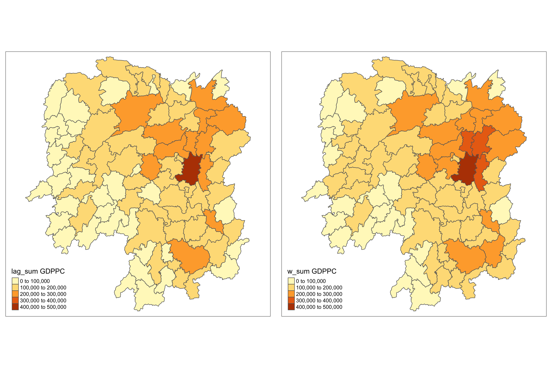
Lastly, qtm() of tmap package is used to plot the lag_sum GDPPC and w_sum_gdppc maps next to each other for quick comparison.

w_sum_gdppc <- qtm(hunan, "w_sum GDPPC")
tmap_arrange(lag_sum_gdppc, w_sum_gdppc, asp=1, ncol=2)