pacman::p_load(sf, raster, spatstat, tmap, tidyverse)2B: 2nd Order Spatial Point Patterns Analysis
In this exercise, we will learn to apply 2nd-order spatial point pattern analysis methods in R, including G, F, K, and L functions, to evaluate spatial point distributions and perform hypothesis testing using the spatstat package.
1 Exercise 2B Reference
R for Geospatial Data Science and Analytics - 5 2nd Order Spatial Point Patterns Analysis Methods
2 Overview
Spatial Point Pattern Analysis is the evaluation of the pattern or distribution, of a set of points on a surface. The point can be location of:
- events such as crime, traffic accident and disease onset, or
- business services (coffee and fastfood outlets) or facilities such as childcare and eldercare.
Using appropriate functions of spatstat, this hands-on exercise aims to discover the spatial point processes of childecare centres in Singapore.
The specific questions we would like to answer are as follows:
-
are the childcare centres in Singapore randomly distributed
throughout the country?
- if the answer is not, then the next logical question is where are the locations with higher concentration of childcare centres?
This hands-on exercise continues from Hands-on Exercise 2A
3 Learning Outcome
-
Importing and managing geospatial data using
sfandspatstatpackages. -
Converting spatial data formats from
sftospatstat’spppformat. - Handling and correcting duplicate spatial points in datasets.
-
Defining and applying spatial windows (
owinobjects) for focused analysis. - Conducting 2nd-order spatial point pattern analyses using G, F, K, and L functions.
- Performing Monte Carlo simulations and hypothesis testing to assess spatial randomness.
- Visualizing spatial patterns and statistical results using appropriate plotting functions.
4 The Data
| Dataset | Description | Source | Format |
|---|---|---|---|
| CHILDCARE | Point data containing location and attributes of childcare centers. | Data.gov.sg | GeoJSON |
| MP14_SUBZONE_WEB_PL | Polygon data with URA 2014 Master Plan Planning Subzone boundaries. | Data.gov.sg | ESRI Shapefile |
| CoastalOutline | Polygon data representing Singapore’s national boundary. | Singapore Land Authority (SLA) | ESRI Shapefile |
5 Installing and Loading the R Packages
The following R packages will be used in this exercise:
| Package | Purpose | Use Case in Exercise |
|---|---|---|
| sf | Imports, manages, and processes vector-based geospatial data. | Handling vector geospatial data in R. |
| spatstat | Provides tools for point pattern analysis. | Performing 1st- and 2nd-order spatial point pattern analysis and deriving kernel density estimation (KDE). |
| raster | Reads, writes, and manipulates gridded spatial data (raster). |
Converting image outputs from spatstat into
raster format.
|
| maptools | Offers tools for manipulating geographic data. |
Converting spatial objects into ppp format for
use with spatstat.
|
| tmap | Creates static and interactive thematic maps using cartographic quality elements. | Plotting static and interactive point pattern maps. |
To install and load these packages in R, use the following code:
6 Reproducibility
As this document involves Monte Carlo simulations, we will set the seed to ensure reproducibility
set.seed(1234)7 Spatial Data Wrangling
7.1 Importing the Spatial Data
To import the three geographical datasets, we will use
st_read() from sf.
childcare_sf <- st_read("data/child-care-services-geojson.geojson")Reading layer `child-care-services-geojson' from data source
`/Users/walter/code/isss626/isss626-gaa/Hands-on_Ex/Hands-on_Ex02/data/child-care-services-geojson.geojson'
using driver `GeoJSON'
Simple feature collection with 1545 features and 2 fields
Geometry type: POINT
Dimension: XYZ
Bounding box: xmin: 103.6824 ymin: 1.248403 xmax: 103.9897 ymax: 1.462134
z_range: zmin: 0 zmax: 0
Geodetic CRS: WGS 84sg_sf <- st_read(dsn = "data", layer="CostalOutline")Reading layer `CostalOutline' from data source
`/Users/walter/code/isss626/isss626-gaa/Hands-on_Ex/Hands-on_Ex02/data'
using driver `ESRI Shapefile'
Simple feature collection with 60 features and 4 fields
Geometry type: POLYGON
Dimension: XY
Bounding box: xmin: 2663.926 ymin: 16357.98 xmax: 56047.79 ymax: 50244.03
Projected CRS: SVY21mpsz_sf <- st_read(dsn = "data",
layer = "MP14_SUBZONE_WEB_PL")Reading layer `MP14_SUBZONE_WEB_PL' from data source
`/Users/walter/code/isss626/isss626-gaa/Hands-on_Ex/Hands-on_Ex02/data'
using driver `ESRI Shapefile'
Simple feature collection with 323 features and 15 fields
Geometry type: MULTIPOLYGON
Dimension: XY
Bounding box: xmin: 2667.538 ymin: 15748.72 xmax: 56396.44 ymax: 50256.33
Projected CRS: SVY217.2 Inspect and Reproject to Same Projection System
Before we can use these data for analysis, it is important for us to ensure that they are projected in same projection system.
First, we check the childcare dataset.
st_crs(childcare_sf)Coordinate Reference System:
User input: WGS 84
wkt:
GEOGCRS["WGS 84",
DATUM["World Geodetic System 1984",
ELLIPSOID["WGS 84",6378137,298.257223563,
LENGTHUNIT["metre",1]]],
PRIMEM["Greenwich",0,
ANGLEUNIT["degree",0.0174532925199433]],
CS[ellipsoidal,2],
AXIS["geodetic latitude (Lat)",north,
ORDER[1],
ANGLEUNIT["degree",0.0174532925199433]],
AXIS["geodetic longitude (Lon)",east,
ORDER[2],
ANGLEUNIT["degree",0.0174532925199433]],
ID["EPSG",4326]]This dataset is using the WGS84 crs. We will reproject all the dataset to SVY21 crs for standardization and analysis.
childcare_sf <- st_transform(childcare_sf , crs = 3414)
st_crs(childcare_sf)
Coordinate Reference System:
User input: EPSG:3414
wkt:
PROJCRS["SVY21 / Singapore TM",
BASEGEOGCRS["SVY21",
DATUM["SVY21",
ELLIPSOID["WGS 84",6378137,298.257223563,
LENGTHUNIT["metre",1]]],
PRIMEM["Greenwich",0,
ANGLEUNIT["degree",0.0174532925199433]],
ID["EPSG",4757]],
CONVERSION["Singapore Transverse Mercator",
METHOD["Transverse Mercator",
ID["EPSG",9807]],
PARAMETER["Latitude of natural origin",1.36666666666667,
ANGLEUNIT["degree",0.0174532925199433],
ID["EPSG",8801]],
PARAMETER["Longitude of natural origin",103.833333333333,
ANGLEUNIT["degree",0.0174532925199433],
ID["EPSG",8802]],
PARAMETER["Scale factor at natural origin",1,
SCALEUNIT["unity",1],
ID["EPSG",8805]],
PARAMETER["False easting",28001.642,
LENGTHUNIT["metre",1],
ID["EPSG",8806]],
PARAMETER["False northing",38744.572,
LENGTHUNIT["metre",1],
ID["EPSG",8807]]],
CS[Cartesian,2],
AXIS["northing (N)",north,
ORDER[1],
LENGTHUNIT["metre",1]],
AXIS["easting (E)",east,
ORDER[2],
LENGTHUNIT["metre",1]],
USAGE[
SCOPE["Cadastre, engineering survey, topographic mapping."],
AREA["Singapore - onshore and offshore."],
BBOX[1.13,103.59,1.47,104.07]],
ID["EPSG",3414]]The childcare dataset has been reprojected to SVY21 successfully.
Next, we inspect the Coastal Outline dataset.
st_crs(sg_sf)Coordinate Reference System:
User input: SVY21
wkt:
PROJCRS["SVY21",
BASEGEOGCRS["SVY21[WGS84]",
DATUM["World Geodetic System 1984",
ELLIPSOID["WGS 84",6378137,298.257223563,
LENGTHUNIT["metre",1]],
ID["EPSG",6326]],
PRIMEM["Greenwich",0,
ANGLEUNIT["Degree",0.0174532925199433]]],
CONVERSION["unnamed",
METHOD["Transverse Mercator",
ID["EPSG",9807]],
PARAMETER["Latitude of natural origin",1.36666666666667,
ANGLEUNIT["Degree",0.0174532925199433],
ID["EPSG",8801]],
PARAMETER["Longitude of natural origin",103.833333333333,
ANGLEUNIT["Degree",0.0174532925199433],
ID["EPSG",8802]],
PARAMETER["Scale factor at natural origin",1,
SCALEUNIT["unity",1],
ID["EPSG",8805]],
PARAMETER["False easting",28001.642,
LENGTHUNIT["metre",1],
ID["EPSG",8806]],
PARAMETER["False northing",38744.572,
LENGTHUNIT["metre",1],
ID["EPSG",8807]]],
CS[Cartesian,2],
AXIS["(E)",east,
ORDER[1],
LENGTHUNIT["metre",1,
ID["EPSG",9001]]],
AXIS["(N)",north,
ORDER[2],
LENGTHUNIT["metre",1,
ID["EPSG",9001]]]]
Notice that this dataset is using SVY21 crs, however the ID
provided is EPSG:9001 does not match the intended ID,
EPSG:3414 of SVY21. In this case, we will set the crs
to the correct ID using the code block below.
sg_sf <- st_set_crs(sg_sf, 3414)
st_crs(sg_sf)
Coordinate Reference System:
User input: EPSG:3414
wkt:
PROJCRS["SVY21 / Singapore TM",
BASEGEOGCRS["SVY21",
DATUM["SVY21",
ELLIPSOID["WGS 84",6378137,298.257223563,
LENGTHUNIT["metre",1]]],
PRIMEM["Greenwich",0,
ANGLEUNIT["degree",0.0174532925199433]],
ID["EPSG",4757]],
CONVERSION["Singapore Transverse Mercator",
METHOD["Transverse Mercator",
ID["EPSG",9807]],
PARAMETER["Latitude of natural origin",1.36666666666667,
ANGLEUNIT["degree",0.0174532925199433],
ID["EPSG",8801]],
PARAMETER["Longitude of natural origin",103.833333333333,
ANGLEUNIT["degree",0.0174532925199433],
ID["EPSG",8802]],
PARAMETER["Scale factor at natural origin",1,
SCALEUNIT["unity",1],
ID["EPSG",8805]],
PARAMETER["False easting",28001.642,
LENGTHUNIT["metre",1],
ID["EPSG",8806]],
PARAMETER["False northing",38744.572,
LENGTHUNIT["metre",1],
ID["EPSG",8807]]],
CS[Cartesian,2],
AXIS["northing (N)",north,
ORDER[1],
LENGTHUNIT["metre",1]],
AXIS["easting (E)",east,
ORDER[2],
LENGTHUNIT["metre",1]],
USAGE[
SCOPE["Cadastre, engineering survey, topographic mapping."],
AREA["Singapore - onshore and offshore."],
BBOX[1.13,103.59,1.47,104.07]],
ID["EPSG",3414]]Similarly, we will inspect the Master Plan Subzone Dataset.
st_crs(mpsz_sf)Coordinate Reference System:
User input: SVY21
wkt:
PROJCRS["SVY21",
BASEGEOGCRS["SVY21[WGS84]",
DATUM["World Geodetic System 1984",
ELLIPSOID["WGS 84",6378137,298.257223563,
LENGTHUNIT["metre",1]],
ID["EPSG",6326]],
PRIMEM["Greenwich",0,
ANGLEUNIT["Degree",0.0174532925199433]]],
CONVERSION["unnamed",
METHOD["Transverse Mercator",
ID["EPSG",9807]],
PARAMETER["Latitude of natural origin",1.36666666666667,
ANGLEUNIT["Degree",0.0174532925199433],
ID["EPSG",8801]],
PARAMETER["Longitude of natural origin",103.833333333333,
ANGLEUNIT["Degree",0.0174532925199433],
ID["EPSG",8802]],
PARAMETER["Scale factor at natural origin",1,
SCALEUNIT["unity",1],
ID["EPSG",8805]],
PARAMETER["False easting",28001.642,
LENGTHUNIT["metre",1],
ID["EPSG",8806]],
PARAMETER["False northing",38744.572,
LENGTHUNIT["metre",1],
ID["EPSG",8807]]],
CS[Cartesian,2],
AXIS["(E)",east,
ORDER[1],
LENGTHUNIT["metre",1,
ID["EPSG",9001]]],
AXIS["(N)",north,
ORDER[2],
LENGTHUNIT["metre",1,
ID["EPSG",9001]]]]
Since the ID is also EPSG:9001, we will set the crs
to EPSG:3414 too.
mpsz_sf <- st_set_crs(mpsz_sf, 3414)
st_crs(mpsz_sf)
Coordinate Reference System:
User input: EPSG:3414
wkt:
PROJCRS["SVY21 / Singapore TM",
BASEGEOGCRS["SVY21",
DATUM["SVY21",
ELLIPSOID["WGS 84",6378137,298.257223563,
LENGTHUNIT["metre",1]]],
PRIMEM["Greenwich",0,
ANGLEUNIT["degree",0.0174532925199433]],
ID["EPSG",4757]],
CONVERSION["Singapore Transverse Mercator",
METHOD["Transverse Mercator",
ID["EPSG",9807]],
PARAMETER["Latitude of natural origin",1.36666666666667,
ANGLEUNIT["degree",0.0174532925199433],
ID["EPSG",8801]],
PARAMETER["Longitude of natural origin",103.833333333333,
ANGLEUNIT["degree",0.0174532925199433],
ID["EPSG",8802]],
PARAMETER["Scale factor at natural origin",1,
SCALEUNIT["unity",1],
ID["EPSG",8805]],
PARAMETER["False easting",28001.642,
LENGTHUNIT["metre",1],
ID["EPSG",8806]],
PARAMETER["False northing",38744.572,
LENGTHUNIT["metre",1],
ID["EPSG",8807]]],
CS[Cartesian,2],
AXIS["northing (N)",north,
ORDER[1],
LENGTHUNIT["metre",1]],
AXIS["easting (E)",east,
ORDER[2],
LENGTHUNIT["metre",1]],
USAGE[
SCOPE["Cadastre, engineering survey, topographic mapping."],
AREA["Singapore - onshore and offshore."],
BBOX[1.13,103.59,1.47,104.07]],
ID["EPSG",3414]]8 Mapping the Geospatial Datasets
After checking the referencing system of each geospatial data data frame, it is also useful for us to plot a map to show their spatial patterns.
8.1 Static Map
# add polygon layer of the coastal outline of sg island
tm_shape(sg_sf)+ tm_polygons() +
# add polygon layer of the subzone based on sg masterplan
tm_shape(mpsz_sf) + tm_polygons() +
# add dot layer to show the locations of childcare centres
tm_shape(childcare_sf) + tm_dots() +
tm_layout()
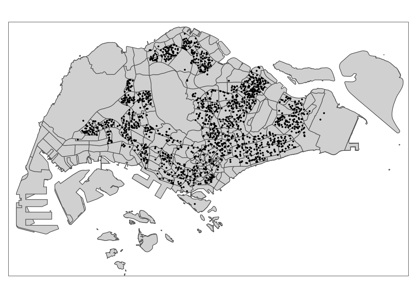
When all the 3 datasets are overlayed together, it shows the locations of childcare centres on the Singapore island. Since all the geospatial layers are within the same map context, it means their referencing system and coordinate values are referred to similar spatial context. This consistency is crucial for accurate geospatial analysis.
8.2 Interactive Map
Alternatively, we can also prepare a pin map by using the code block below.
tmap_mode('view')

# tm_basemap("Esri.WorldGrayCanvas") +
# tm_basemap("OpenStreetMap") +
tm_basemap("Esri.WorldTopoMap") +
tm_shape(childcare_sf) +
tm_dots(alpha = 0.5)tmap_mode('plot')
In interactive mode, tmap uses the Leaflet for R API,
allowing you to freely navigate, zoom, and click on features for
detailed information. You can also change the map’s background
using layers like ESRI.WorldGrayCanvas, OpenStreetMap, and
ESRI.WorldTopoMap, with ESRI.WorldGrayCanvas as the default.
Tip
Remember to switch back to plot mode after interacting to avoid connection issues and limit interactive maps to fewer than 10 in RMarkdown documents for Netlify publishing.
9 Geospatial Data Wrangling
While simple feature data frames are becoming more popular compared
to sp’s Spatial* classes, many geospatial analysis
packages still require data in the Spatial* format. This section
will show you how to convert a simple feature data frame to
sp’s Spatial* class.
9.1 Converting sf data frames to sp’s Spatial* class
The code block below uses
as_Spatial()
of sf package to convert the three geospatial
data from simple feature data frame to sp’s Spatial* class.
childcare <- as_Spatial(childcare_sf)
mpsz <- as_Spatial(mpsz_sf)
sg <- as_Spatial(sg_sf)
After the sf dataframe to sp Spatial* conversion, let’s inspect the Spatial* classes.
childcareclass : SpatialPointsDataFrame
features : 1545
extent : 11203.01, 45404.24, 25667.6, 49300.88 (xmin, xmax, ymin, ymax)
crs : +proj=tmerc +lat_0=1.36666666666667 +lon_0=103.833333333333 +k=1 +x_0=28001.642 +y_0=38744.572 +ellps=WGS84 +towgs84=0,0,0,0,0,0,0 +units=m +no_defs
variables : 2
names : Name, Description
min values : kml_1, <center><table><tr><th colspan='2' align='center'><em>Attributes</em></th></tr><tr bgcolor="#E3E3F3"> <th>ADDRESSBLOCKHOUSENUMBER</th> <td></td> </tr><tr bgcolor=""> <th>ADDRESSBUILDINGNAME</th> <td></td> </tr><tr bgcolor="#E3E3F3"> <th>ADDRESSPOSTALCODE</th> <td>018989</td> </tr><tr bgcolor=""> <th>ADDRESSSTREETNAME</th> <td>1, MARINA BOULEVARD, #B1 - 01, ONE MARINA BOULEVARD, SINGAPORE 018989</td> </tr><tr bgcolor="#E3E3F3"> <th>ADDRESSTYPE</th> <td></td> </tr><tr bgcolor=""> <th>DESCRIPTION</th> <td></td> </tr><tr bgcolor="#E3E3F3"> <th>HYPERLINK</th> <td></td> </tr><tr bgcolor=""> <th>LANDXADDRESSPOINT</th> <td>0</td> </tr><tr bgcolor="#E3E3F3"> <th>LANDYADDRESSPOINT</th> <td>0</td> </tr><tr bgcolor=""> <th>NAME</th> <td>THE LITTLE SKOOL-HOUSE INTERNATIONAL PTE. LTD.</td> </tr><tr bgcolor="#E3E3F3"> <th>PHOTOURL</th> <td></td> </tr><tr bgcolor=""> <th>ADDRESSFLOORNUMBER</th> <td></td> </tr><tr bgcolor="#E3E3F3"> <th>INC_CRC</th> <td>08F73931F4A691F4</td> </tr><tr bgcolor=""> <th>FMEL_UPD_D</th> <td>20200826094036</td> </tr><tr bgcolor="#E3E3F3"> <th>ADDRESSUNITNUMBER</th> <td></td> </tr></table></center>
max values : kml_999, <center><table><tr><th colspan='2' align='center'><em>Attributes</em></th></tr><tr bgcolor="#E3E3F3"> <th>ADDRESSBLOCKHOUSENUMBER</th> <td></td> </tr><tr bgcolor=""> <th>ADDRESSBUILDINGNAME</th> <td></td> </tr><tr bgcolor="#E3E3F3"> <th>ADDRESSPOSTALCODE</th> <td>829646</td> </tr><tr bgcolor=""> <th>ADDRESSSTREETNAME</th> <td>200, PONGGOL SEVENTEENTH AVENUE, SINGAPORE 829646</td> </tr><tr bgcolor="#E3E3F3"> <th>ADDRESSTYPE</th> <td></td> </tr><tr bgcolor=""> <th>DESCRIPTION</th> <td>Child Care Services</td> </tr><tr bgcolor="#E3E3F3"> <th>HYPERLINK</th> <td></td> </tr><tr bgcolor=""> <th>LANDXADDRESSPOINT</th> <td>0</td> </tr><tr bgcolor="#E3E3F3"> <th>LANDYADDRESSPOINT</th> <td>0</td> </tr><tr bgcolor=""> <th>NAME</th> <td>RAFFLES KIDZ @ PUNGGOL PTE LTD</td> </tr><tr bgcolor="#E3E3F3"> <th>PHOTOURL</th> <td></td> </tr><tr bgcolor=""> <th>ADDRESSFLOORNUMBER</th> <td></td> </tr><tr bgcolor="#E3E3F3"> <th>INC_CRC</th> <td>379D017BF244B0FA</td> </tr><tr bgcolor=""> <th>FMEL_UPD_D</th> <td>20200826094036</td> </tr><tr bgcolor="#E3E3F3"> <th>ADDRESSUNITNUMBER</th> <td></td> </tr></table></center> mpszclass : SpatialPolygonsDataFrame
features : 323
extent : 2667.538, 56396.44, 15748.72, 50256.33 (xmin, xmax, ymin, ymax)
crs : +proj=tmerc +lat_0=1.36666666666667 +lon_0=103.833333333333 +k=1 +x_0=28001.642 +y_0=38744.572 +ellps=WGS84 +towgs84=0,0,0,0,0,0,0 +units=m +no_defs
variables : 15
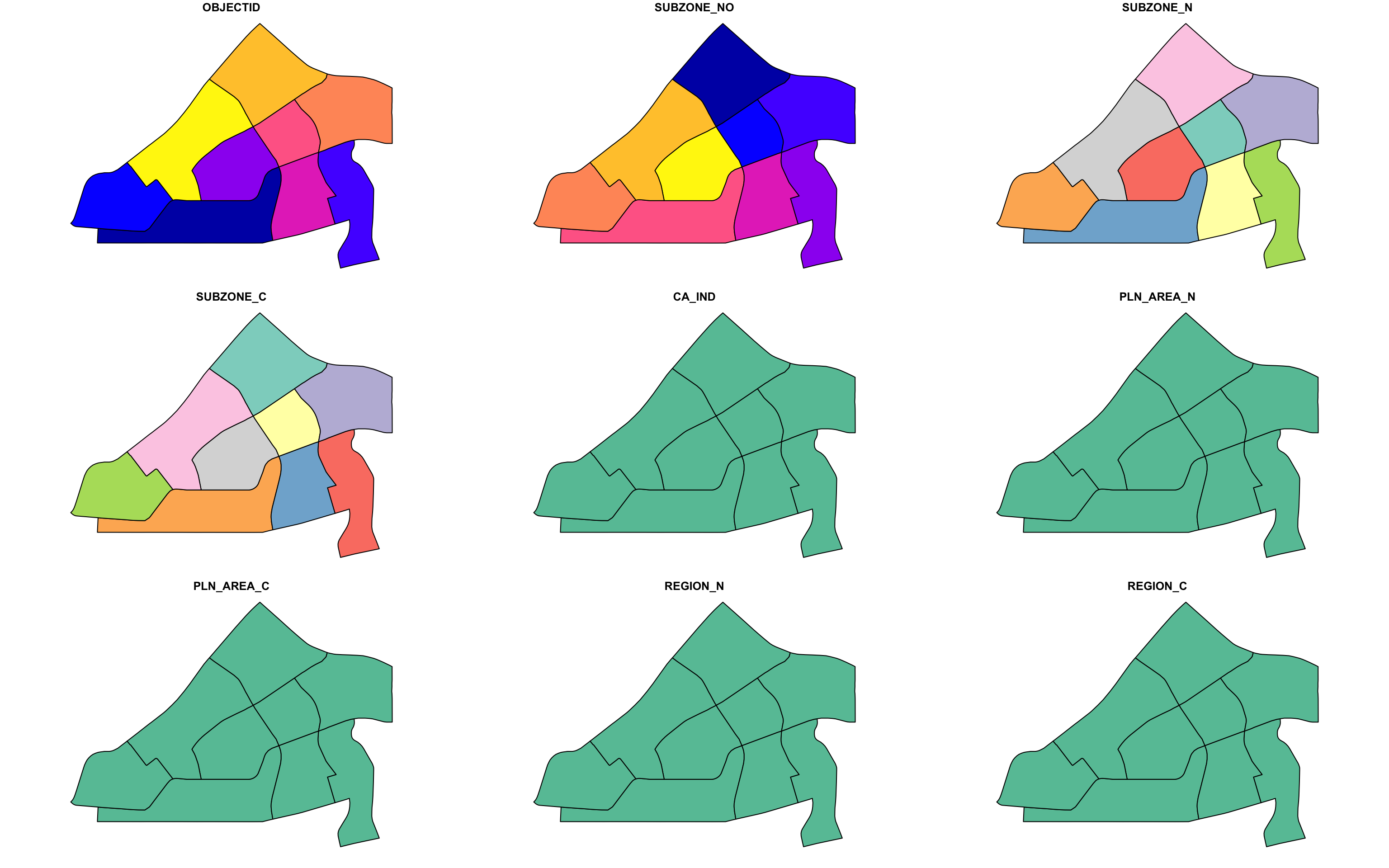
names : OBJECTID, SUBZONE_NO, SUBZONE_N, SUBZONE_C, CA_IND, PLN_AREA_N, PLN_AREA_C, REGION_N, REGION_C, INC_CRC, FMEL_UPD_D, X_ADDR, Y_ADDR, SHAPE_Leng, SHAPE_Area
min values : 1, 1, ADMIRALTY, AMSZ01, N, ANG MO KIO, AM, CENTRAL REGION, CR, 00F5E30B5C9B7AD8, 16409, 5092.8949, 19579.069, 871.554887798, 39437.9352703
max values : 323, 17, YUNNAN, YSSZ09, Y, YISHUN, YS, WEST REGION, WR, FFCCF172717C2EAF, 16409, 50424.7923, 49552.7904, 68083.9364708, 69748298.792 sgclass : SpatialPolygonsDataFrame
features : 60
extent : 2663.926, 56047.79, 16357.98, 50244.03 (xmin, xmax, ymin, ymax)
crs : +proj=tmerc +lat_0=1.36666666666667 +lon_0=103.833333333333 +k=1 +x_0=28001.642 +y_0=38744.572 +ellps=WGS84 +towgs84=0,0,0,0,0,0,0 +units=m +no_defs
variables : 4
names : GDO_GID, MSLINK, MAPID, COSTAL_NAM
min values : 1, 1, 0, ISLAND LINK
max values : 60, 67, 0, SINGAPORE - MAIN ISLAND The geospatial data have been converted into their respective sp’s Spatial* classes.
9.2 Converting the Spatial* Class into Generic sp Format
spatstat requires the analytical data in ppp object form. There is no straightforward way to convert a Spatial* classes into ppp object. We need to convert the Spatial classes* into Spatial object first.
Tip
ppp refers to
planar point pattern. It is used to represent
spatial point patterns in spatstat; it contains
the event locations with possibly associated marks, and the
observation window where the events occur.
see Chapter 18 The spatstat package | Spatial Statistics for Data Science: Theory and Practice with R
The codes block below converts the Spatial* classes into generic sp objects.
childcare_sp <- as(childcare, "SpatialPoints")
sg_sp <- as(sg, "SpatialPolygons")
Next, we can display the sp objects properties.
childcare_spclass : SpatialPoints
features : 1545
extent : 11203.01, 45404.24, 25667.6, 49300.88 (xmin, xmax, ymin, ymax)
crs : +proj=tmerc +lat_0=1.36666666666667 +lon_0=103.833333333333 +k=1 +x_0=28001.642 +y_0=38744.572 +ellps=WGS84 +towgs84=0,0,0,0,0,0,0 +units=m +no_defs sg_spclass : SpatialPolygons
features : 60
extent : 2663.926, 56047.79, 16357.98, 50244.03 (xmin, xmax, ymin, ymax)
crs : +proj=tmerc +lat_0=1.36666666666667 +lon_0=103.833333333333 +k=1 +x_0=28001.642 +y_0=38744.572 +ellps=WGS84 +towgs84=0,0,0,0,0,0,0 +units=m +no_defs
Let’s further inspect the differences between Spatial* classes and
generic sp object with the example of childcare and
childcare_sp object.
head(childcare) Name
1 kml_1
2 kml_2
3 kml_3
4 kml_4
5 kml_5
6 kml_6
Description
1 <center><table><tr><th colspan='2' align='center'><em>Attributes</em></th></tr><tr bgcolor="#E3E3F3"> <th>ADDRESSBLOCKHOUSENUMBER</th> <td></td> </tr><tr bgcolor=""> <th>ADDRESSBUILDINGNAME</th> <td></td> </tr><tr bgcolor="#E3E3F3"> <th>ADDRESSPOSTALCODE</th> <td>760742</td> </tr><tr bgcolor=""> <th>ADDRESSSTREETNAME</th> <td>742, YISHUN AVENUE 5, #01 - 470, SINGAPORE 760742</td> </tr><tr bgcolor="#E3E3F3"> <th>ADDRESSTYPE</th> <td></td> </tr><tr bgcolor=""> <th>DESCRIPTION</th> <td>Child Care Services</td> </tr><tr bgcolor="#E3E3F3"> <th>HYPERLINK</th> <td></td> </tr><tr bgcolor=""> <th>LANDXADDRESSPOINT</th> <td>0</td> </tr><tr bgcolor="#E3E3F3"> <th>LANDYADDRESSPOINT</th> <td>0</td> </tr><tr bgcolor=""> <th>NAME</th> <td>AVERBEL CHILD DEVELOPMENT CENTRE PTE LTD</td> </tr><tr bgcolor="#E3E3F3"> <th>PHOTOURL</th> <td></td> </tr><tr bgcolor=""> <th>ADDRESSFLOORNUMBER</th> <td></td> </tr><tr bgcolor="#E3E3F3"> <th>INC_CRC</th> <td>AEA27114446235CE</td> </tr><tr bgcolor=""> <th>FMEL_UPD_D</th> <td>20200826094036</td> </tr><tr bgcolor="#E3E3F3"> <th>ADDRESSUNITNUMBER</th> <td></td> </tr></table></center>
2 <center><table><tr><th colspan='2' align='center'><em>Attributes</em></th></tr><tr bgcolor="#E3E3F3"> <th>ADDRESSBLOCKHOUSENUMBER</th> <td></td> </tr><tr bgcolor=""> <th>ADDRESSBUILDINGNAME</th> <td></td> </tr><tr bgcolor="#E3E3F3"> <th>ADDRESSPOSTALCODE</th> <td>159053</td> </tr><tr bgcolor=""> <th>ADDRESSSTREETNAME</th> <td>20, LENGKOK BAHRU, #02 - 05, SINGAPORE 159053</td> </tr><tr bgcolor="#E3E3F3"> <th>ADDRESSTYPE</th> <td></td> </tr><tr bgcolor=""> <th>DESCRIPTION</th> <td>Child Care Services</td> </tr><tr bgcolor="#E3E3F3"> <th>HYPERLINK</th> <td></td> </tr><tr bgcolor=""> <th>LANDXADDRESSPOINT</th> <td>0</td> </tr><tr bgcolor="#E3E3F3"> <th>LANDYADDRESSPOINT</th> <td>0</td> </tr><tr bgcolor=""> <th>NAME</th> <td>AWWA LTD.</td> </tr><tr bgcolor="#E3E3F3"> <th>PHOTOURL</th> <td></td> </tr><tr bgcolor=""> <th>ADDRESSFLOORNUMBER</th> <td></td> </tr><tr bgcolor="#E3E3F3"> <th>INC_CRC</th> <td>86B24416FB1663C6</td> </tr><tr bgcolor=""> <th>FMEL_UPD_D</th> <td>20200826094036</td> </tr><tr bgcolor="#E3E3F3"> <th>ADDRESSUNITNUMBER</th> <td></td> </tr></table></center>
3 <center><table><tr><th colspan='2' align='center'><em>Attributes</em></th></tr><tr bgcolor="#E3E3F3"> <th>ADDRESSBLOCKHOUSENUMBER</th> <td></td> </tr><tr bgcolor=""> <th>ADDRESSBUILDINGNAME</th> <td></td> </tr><tr bgcolor="#E3E3F3"> <th>ADDRESSPOSTALCODE</th> <td>556912</td> </tr><tr bgcolor=""> <th>ADDRESSSTREETNAME</th> <td>22, LI HWAN VIEW, GOLDEN HILL ESTATE, SINGAPORE 556912</td> </tr><tr bgcolor="#E3E3F3"> <th>ADDRESSTYPE</th> <td></td> </tr><tr bgcolor=""> <th>DESCRIPTION</th> <td>Child Care Services</td> </tr><tr bgcolor="#E3E3F3"> <th>HYPERLINK</th> <td></td> </tr><tr bgcolor=""> <th>LANDXADDRESSPOINT</th> <td>0</td> </tr><tr bgcolor="#E3E3F3"> <th>LANDYADDRESSPOINT</th> <td>0</td> </tr><tr bgcolor=""> <th>NAME</th> <td>BABIES BY-THE-PARK PTE. LTD.</td> </tr><tr bgcolor="#E3E3F3"> <th>PHOTOURL</th> <td></td> </tr><tr bgcolor=""> <th>ADDRESSFLOORNUMBER</th> <td></td> </tr><tr bgcolor="#E3E3F3"> <th>INC_CRC</th> <td>F971CBBA973E1AE5</td> </tr><tr bgcolor=""> <th>FMEL_UPD_D</th> <td>20200826094036</td> </tr><tr bgcolor="#E3E3F3"> <th>ADDRESSUNITNUMBER</th> <td></td> </tr></table></center>
4 <center><table><tr><th colspan='2' align='center'><em>Attributes</em></th></tr><tr bgcolor="#E3E3F3"> <th>ADDRESSBLOCKHOUSENUMBER</th> <td></td> </tr><tr bgcolor=""> <th>ADDRESSBUILDINGNAME</th> <td></td> </tr><tr bgcolor="#E3E3F3"> <th>ADDRESSPOSTALCODE</th> <td>569139</td> </tr><tr bgcolor=""> <th>ADDRESSSTREETNAME</th> <td>3, ANG MO KIO STREET 62, #01 - 36, LINK@AMK, SINGAPORE 569139</td> </tr><tr bgcolor="#E3E3F3"> <th>ADDRESSTYPE</th> <td></td> </tr><tr bgcolor=""> <th>DESCRIPTION</th> <td>Child Care Services</td> </tr><tr bgcolor="#E3E3F3"> <th>HYPERLINK</th> <td></td> </tr><tr bgcolor=""> <th>LANDXADDRESSPOINT</th> <td>0</td> </tr><tr bgcolor="#E3E3F3"> <th>LANDYADDRESSPOINT</th> <td>0</td> </tr><tr bgcolor=""> <th>NAME</th> <td>Baby Elk Infant Care Pte Ltd</td> </tr><tr bgcolor="#E3E3F3"> <th>PHOTOURL</th> <td></td> </tr><tr bgcolor=""> <th>ADDRESSFLOORNUMBER</th> <td></td> </tr><tr bgcolor="#E3E3F3"> <th>INC_CRC</th> <td>86A4F25D1C7C9D85</td> </tr><tr bgcolor=""> <th>FMEL_UPD_D</th> <td>20200826094036</td> </tr><tr bgcolor="#E3E3F3"> <th>ADDRESSUNITNUMBER</th> <td></td> </tr></table></center>
5 <center><table><tr><th colspan='2' align='center'><em>Attributes</em></th></tr><tr bgcolor="#E3E3F3"> <th>ADDRESSBLOCKHOUSENUMBER</th> <td></td> </tr><tr bgcolor=""> <th>ADDRESSBUILDINGNAME</th> <td></td> </tr><tr bgcolor="#E3E3F3"> <th>ADDRESSPOSTALCODE</th> <td>467961</td> </tr><tr bgcolor=""> <th>ADDRESSSTREETNAME</th> <td>22A, KEW DRIVE, SINGAPORE 467961</td> </tr><tr bgcolor="#E3E3F3"> <th>ADDRESSTYPE</th> <td></td> </tr><tr bgcolor=""> <th>DESCRIPTION</th> <td>Child Care Services</td> </tr><tr bgcolor="#E3E3F3"> <th>HYPERLINK</th> <td></td> </tr><tr bgcolor=""> <th>LANDXADDRESSPOINT</th> <td>0</td> </tr><tr bgcolor="#E3E3F3"> <th>LANDYADDRESSPOINT</th> <td>0</td> </tr><tr bgcolor=""> <th>NAME</th> <td>BABYPLANET MONTESSORI PTE. LTD.</td> </tr><tr bgcolor="#E3E3F3"> <th>PHOTOURL</th> <td></td> </tr><tr bgcolor=""> <th>ADDRESSFLOORNUMBER</th> <td></td> </tr><tr bgcolor="#E3E3F3"> <th>INC_CRC</th> <td>CFE3F056F8171C7B</td> </tr><tr bgcolor=""> <th>FMEL_UPD_D</th> <td>20200826094036</td> </tr><tr bgcolor="#E3E3F3"> <th>ADDRESSUNITNUMBER</th> <td></td> </tr></table></center>
6 <center><table><tr><th colspan='2' align='center'><em>Attributes</em></th></tr><tr bgcolor="#E3E3F3"> <th>ADDRESSBLOCKHOUSENUMBER</th> <td></td> </tr><tr bgcolor=""> <th>ADDRESSBUILDINGNAME</th> <td></td> </tr><tr bgcolor="#E3E3F3"> <th>ADDRESSPOSTALCODE</th> <td>598523</td> </tr><tr bgcolor=""> <th>ADDRESSSTREETNAME</th> <td>3 Jalan Kakatua, JURONG PARK, SINGAPORE 598523</td> </tr><tr bgcolor="#E3E3F3"> <th>ADDRESSTYPE</th> <td></td> </tr><tr bgcolor=""> <th>DESCRIPTION</th> <td>Child Care Services</td> </tr><tr bgcolor="#E3E3F3"> <th>HYPERLINK</th> <td></td> </tr><tr bgcolor=""> <th>LANDXADDRESSPOINT</th> <td>0</td> </tr><tr bgcolor="#E3E3F3"> <th>LANDYADDRESSPOINT</th> <td>0</td> </tr><tr bgcolor=""> <th>NAME</th> <td>BAMBINI CHILDCARE LLP</td> </tr><tr bgcolor="#E3E3F3"> <th>PHOTOURL</th> <td></td> </tr><tr bgcolor=""> <th>ADDRESSFLOORNUMBER</th> <td></td> </tr><tr bgcolor="#E3E3F3"> <th>INC_CRC</th> <td>2B4F0B285ED28C4A</td> </tr><tr bgcolor=""> <th>FMEL_UPD_D</th> <td>20200826094036</td> </tr><tr bgcolor="#E3E3F3"> <th>ADDRESSUNITNUMBER</th> <td></td> </tr></table></center>head(childcare_sp)class : SpatialPoints
features : 1
extent : 27976.73, 27976.73, 45716.7, 45716.7 (xmin, xmax, ymin, ymax)
crs : +proj=tmerc +lat_0=1.36666666666667 +lon_0=103.833333333333 +k=1 +x_0=28001.642 +y_0=38744.572 +ellps=WGS84 +towgs84=0,0,0,0,0,0,0 +units=m +no_defs Note that the Spatial* classes contain more attribute data as compared its generic sp object counterpart.
Tip
Differences between Spatial* classes and generic sp object
-
Data Storage: SpatialPoints stores only the coordinates, while SpatialPointsDataFrame stores both coordinates and additional attribute data
-
Functionality: SpatialPointsDataFrame allows for more complex operations and analyses due to the additional data it holds
see Introduction to spatial points in R - Michael T. Hallworth, Ph.D.
9.3 Converting the Generic sp Format into spatstat’s ppp Format
Now, we will use as.ppp() function of
spatstat to convert the spatial data into
spatstat’s ppp object
format.
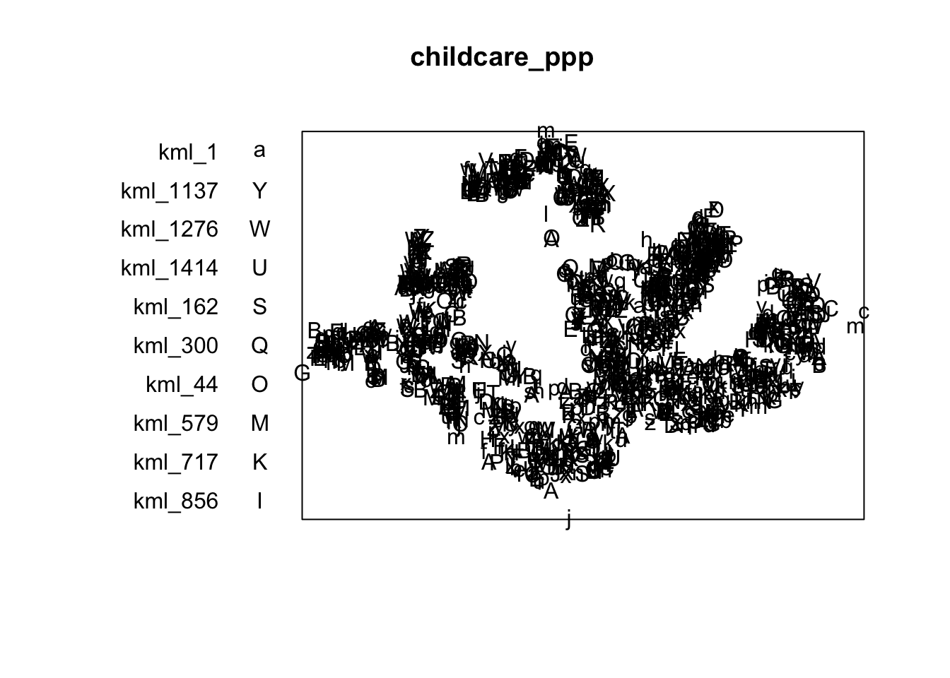
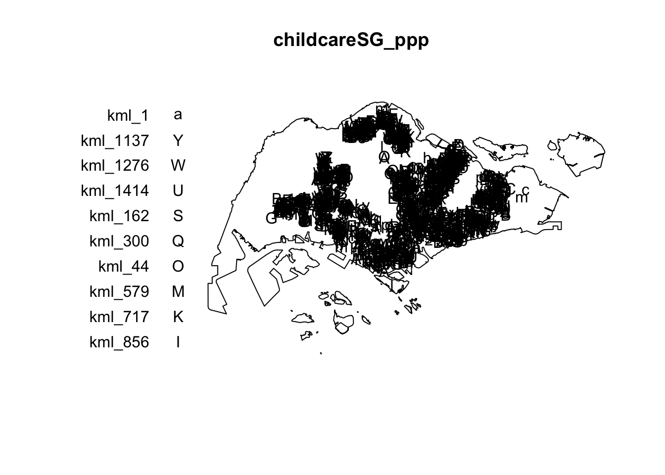
childcare_ppp <- as.ppp(childcare_sf)
childcare_ppp
Marked planar point pattern: 1545 points
marks are of storage type 'character'
window: rectangle = [11203.01, 45404.24] x [25667.6, 49300.88] unitsLet’s examine the difference by plotting childcare_ppp:
plot(childcare_ppp)
We can also view the summary statistics of the newly created ppp object by using the code block below.
summary(childcare_ppp)Marked planar point pattern: 1545 points
Average intensity 1.91145e-06 points per square unit
Coordinates are given to 11 decimal places
marks are of type 'character'
Summary:
Length Class Mode
1545 character character
Window: rectangle = [11203.01, 45404.24] x [25667.6, 49300.88] units
(34200 x 23630 units)
Window area = 808287000 square unitsTip
Be aware of the warning message regarding duplicates. In spatial point pattern analysis, duplicates can be a significant issue. The statistical methods used for analyzing spatial point patterns often assume that the points are distinct and non-coincident.
9.4 Handling Duplicated Points
We can check the duplication in a ppp object by
using the duplicated function with different
configurations.
Tip
The duplicated function has an argument
rule:
-
Default Behavior (
rule = "spatstat"):- Points are considered identical if both their coordinates (like x and y positions) and their marks (additional data or labels attached to the points) are exactly the same.
- This is the strictest check, requiring everything about the points to match.
-
Only Checking Coordinates (
rule = "unmark"):- Points are considered duplicates if their coordinates are the same, regardless of their marks.
- Marks are ignored, so only the positions are compared.
-
Using
deldirPackage (rule = "deldir"):-
Points are considered duplicates based on their
coordinates, but the comparison is done using a specific
method (
duplicatedxy) from thedeldirpackage. -
This approach ensures the check is consistent with other
functions in the
deldirpackage, which is often used for spatial data analysis (like creating Delaunay triangulations).
-
Points are considered duplicates based on their
coordinates, but the comparison is done using a specific
method (
In other words,
-
rule = "spatstat": Strict check (coordinates and marks). -
rule = "unmark": Less strict (coordinates only). -
rule = "deldir": Coordinate check, consistent with thedeldirpackage methods.
see R: Determine Duplicated Points in a Spatial Point Pattern
# duplicated(childcare_ppp)
# any(duplicated(childcare_ppp))
rules <- c("spatstat", "deldir", "unmark")

duplicate_counts <- list()
for (rule in rules) {
  duplicates <- duplicated(childcare_ppp, rule = rule)
  num_duplicates <- sum(duplicates)
  duplicate_counts[[rule]] <- num_duplicates
}

print(duplicate_counts)
$spatstat
[1] 0
$deldir
[1] 0
$unmark
[1] 74Note
Note that this behavior happens because the data contains marked points with the same coordinates but different properties.
Upon manual inspection, a set of example is “39, WOODLANDS CLOSE, #01 - 62, MEGA@WOODLANDS, SINGAPORE 737856” and “39, WOODLANDS CLOSE, #01 - 59, MEGA@WOODLANDS, SINGAPORE 737856”.
These are 2 childcare centres that resides in the same building. Thus, it can only be picked up using the “unmark” rule which only examine for exact match of the point coordinate only.
To count the number of
coincident points, we will use the multiplicity() function as shown
in the code block below. see
R: Multiplicity
for more info.
multiplicity(childcare_ppp)If we want to know how many locations have more than one point event:
sum(multiplicity(childcare_ppp) > 1)[1] 0# double check
coincident_points <- duplicated(childcare_ppp, rule="unmark")
coincident_coordinates <- childcare_ppp[coincident_points]
print(coincident_coordinates)Marked planar point pattern: 74 points
marks are of storage type 'character'
window: rectangle = [11203.01, 45404.24] x [25667.6, 49300.88] unitsThe output shows that there are 74 duplicated point events.
9.5 How to Spot Duplicate Points on the Map
There are three ways to overcome this problem. The easiest way is to delete the duplicates. But, that will also mean that some useful point events will be lost.
The second solution is use jittering, which will add a small perturbation to the duplicate points so that they do not occupy the exact same space.
The third solution is to make each point “unique” and then attach the duplicates of the points to the patterns as marks, as attributes of the points. Then you would need analytical techniques that take into account these marks.
9.5.1 Jittering
The code block below implements the jittering approach.
childcare_ppp_jit <- rjitter(childcare_ppp,
                             retry=TRUE,
                             nsim=1,
                             drop=TRUE)

plot(childcare_ppp_jit, pch = 16, cex = 0.5, main = "Jittered Points")
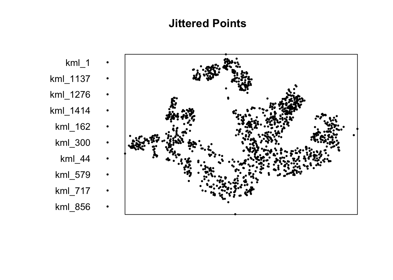
any(duplicated(childcare_ppp_jit))[1] FALSE9.6 Creating owin Object
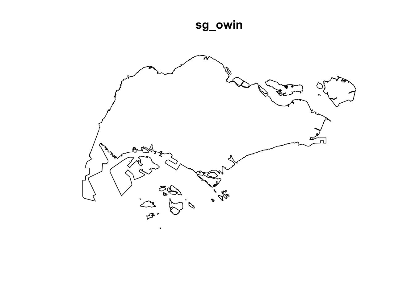
When analysing spatial point patterns, it is a good practice to confine the analysis with a geographical area like Singapore boundary. In spatstat, an object called owin is specially designed to represent this polygonal region.
The code block below is used to covert sg SpatialPolygon object into owin object of spatstat.
sg_owin <- as.owin(sg_sf)
The output object can be displayed by using
plot()
function:
plot(sg_owin)
And using
summary()
function of Base R:
summary(sg_owin)Window: polygonal boundary
50 separate polygons (1 hole)
vertices area relative.area
polygon 1 (hole) 30 -7081.18 -9.76e-06
polygon 2 55 82537.90 1.14e-04
polygon 3 90 415092.00 5.72e-04
polygon 4 49 16698.60 2.30e-05
polygon 5 38 24249.20 3.34e-05
polygon 6 976 23344700.00 3.22e-02
polygon 7 721 1927950.00 2.66e-03
polygon 8 1992 9992170.00 1.38e-02
polygon 9 330 1118960.00 1.54e-03
polygon 10 175 925904.00 1.28e-03
polygon 11 115 928394.00 1.28e-03
polygon 12 24 6352.39 8.76e-06
polygon 13 190 202489.00 2.79e-04
polygon 14 37 10170.50 1.40e-05
polygon 15 25 16622.70 2.29e-05
polygon 16 10 2145.07 2.96e-06
polygon 17 66 16184.10 2.23e-05
polygon 18 5195 636837000.00 8.78e-01
polygon 19 76 312332.00 4.31e-04
polygon 20 627 31891300.00 4.40e-02
polygon 21 20 32842.00 4.53e-05
polygon 22 42 55831.70 7.70e-05
polygon 23 67 1313540.00 1.81e-03
polygon 24 734 4690930.00 6.47e-03
polygon 25 16 3194.60 4.40e-06
polygon 26 15 4872.96 6.72e-06
polygon 27 15 4464.20 6.15e-06
polygon 28 14 5466.74 7.54e-06
polygon 29 37 5261.94 7.25e-06
polygon 30 111 662927.00 9.14e-04
polygon 31 69 56313.40 7.76e-05
polygon 32 143 145139.00 2.00e-04
polygon 33 397 2488210.00 3.43e-03
polygon 34 90 115991.00 1.60e-04
polygon 35 98 62682.90 8.64e-05
polygon 36 165 338736.00 4.67e-04
polygon 37 130 94046.50 1.30e-04
polygon 38 93 430642.00 5.94e-04
polygon 39 16 2010.46 2.77e-06
polygon 40 415 3253840.00 4.49e-03
polygon 41 30 10838.20 1.49e-05
polygon 42 53 34400.30 4.74e-05
polygon 43 26 8347.58 1.15e-05
polygon 44 74 58223.40 8.03e-05
polygon 45 327 2169210.00 2.99e-03
polygon 46 177 467446.00 6.44e-04
polygon 47 46 699702.00 9.65e-04
polygon 48 6 16841.00 2.32e-05
polygon 49 13 70087.30 9.66e-05
polygon 50 4 9459.63 1.30e-05
enclosing rectangle: [2663.93, 56047.79] x [16357.98, 50244.03] units
(53380 x 33890 units)
Window area = 725376000 square units
Fraction of frame area: 0.40110 Combining Point Events Object and Owin Object
For the last step of geospatial data wrangling, we will extract childcare events that are located within Singapore by using the code block below.
Important
Since the dataset contains duplicated points, we will use the jittered ppp object for downstream analysis.
childcareSG_ppp <- childcare_ppp_jit[sg_owin]The output object combined both the point and polygon feature in one ppp object class as shown below.
summary(childcareSG_ppp)Marked planar point pattern: 1545 points
Average intensity 2.129929e-06 points per square unit
Coordinates are given to 11 decimal places
marks are of type 'character'
Summary:
Length Class Mode
1545 character character
Window: polygonal boundary
50 separate polygons (1 hole)
                 vertices         area relative.area
polygon 1 (hole)       30     -7081.18     -9.76e-06
polygon 2              55     82537.90      1.14e-04
polygon 3              90    415092.00      5.72e-04
polygon 4              49     16698.60      2.30e-05
polygon 5              38     24249.20      3.34e-05
polygon 6             976  23344700.00      3.22e-02
polygon 7             721   1927950.00      2.66e-03
polygon 8            1992   9992170.00      1.38e-02
polygon 9             330   1118960.00      1.54e-03
polygon 10            175    925904.00      1.28e-03
polygon 11            115    928394.00      1.28e-03
polygon 12             24      6352.39      8.76e-06
polygon 13            190    202489.00      2.79e-04
polygon 14             37     10170.50      1.40e-05
polygon 15             25     16622.70      2.29e-05
polygon 16             10      2145.07      2.96e-06
polygon 17             66     16184.10      2.23e-05
polygon 18           5195 636837000.00      8.78e-01
polygon 19             76    312332.00      4.31e-04
polygon 20            627  31891300.00      4.40e-02
polygon 21             20     32842.00      4.53e-05
polygon 22             42     55831.70      7.70e-05
polygon 23             67   1313540.00      1.81e-03
polygon 24            734   4690930.00      6.47e-03
polygon 25             16      3194.60      4.40e-06
polygon 26             15      4872.96      6.72e-06
polygon 27             15      4464.20      6.15e-06
polygon 28             14      5466.74      7.54e-06
polygon 29             37      5261.94      7.25e-06
polygon 30            111    662927.00      9.14e-04
polygon 31             69     56313.40      7.76e-05
polygon 32            143    145139.00      2.00e-04
polygon 33            397   2488210.00      3.43e-03
polygon 34             90    115991.00      1.60e-04
polygon 35             98     62682.90      8.64e-05
polygon 36            165    338736.00      4.67e-04
polygon 37            130     94046.50      1.30e-04
polygon 38             93    430642.00      5.94e-04
polygon 39             16      2010.46      2.77e-06
polygon 40            415   3253840.00      4.49e-03
polygon 41             30     10838.20      1.49e-05
polygon 42             53     34400.30      4.74e-05
polygon 43             26      8347.58      1.15e-05
polygon 44             74     58223.40      8.03e-05
polygon 45            327   2169210.00      2.99e-03
polygon 46            177    467446.00      6.44e-04
polygon 47             46    699702.00      9.65e-04
polygon 48              6     16841.00      2.32e-05
polygon 49             13     70087.30      9.66e-05
polygon 50              4      9459.63      1.30e-05
enclosing rectangle: [2663.93, 56047.79] x [16357.98, 50244.03] units
                     (53380 x 33890 units)
Window area = 725376000 square units
Fraction of frame area: 0.401plot(childcareSG_ppp)
11 First-order Spatial Point Patterns Analysis
In this section, you will learn how to perform first-order SPPA by using spatstat package. The hands-on exercise will focus on:
- deriving kernel density estimation (KDE) layer for visualising and exploring the intensity of point processes,
- performing Confirmatory Spatial Point Patterns Analysis by using Nearest Neighbour statistics.
11.1 Kernel Density Estimation
In this section, you will learn how to compute the kernel density estimation (KDE) of childcare services in Singapore.
11.1.1 Computing Kernel Density Estimation Using Automatic Bandwidth Selection Method
-
bw.diggle()
automatic bandwidth selection method. Other recommended
methods are
bw.CvL(),
bw.scott()
or
bw.ppl().
-
The smoothing kernel used is gaussian, which is the
default. Other smoothing methods are: “epanechnikov”,
“quartic” or “disc”.
- The intensity estimate is corrected for edge effect bias by using method described by Jones (1993) and Diggle (2010, equation 18.9). The default is FALSE.
kde_childcareSG_bw <- density(childcareSG_ppp,
                              sigma=bw.diggle,
                              edge=TRUE,
                            kernel="gaussian")
The plot() function of Base R is then used to display the kernel density derived.
plot(kde_childcareSG_bw)
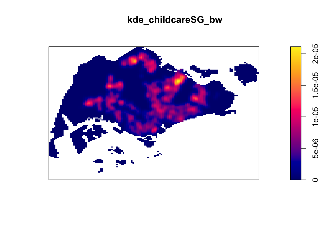
The density values of the output range from 0 to 0.000035 which is way too small to comprehend. This is because the default unit of measurement of SVY21 is in meter. As a result, the density values computed is in “number of points per square meter”.
Before we move on to next section, it is good to know that you can retrieve the bandwidth used to compute the kde layer by using the code block below.
bw <- bw.diggle(childcareSG_ppp)
bw
sigma
414.4576 11.1.2 Rescaling KDE values
rescale.ppp() is used below to convert the unit of
measurement from meter to kilometer:
childcareSG_ppp.km <- rescale.ppp(childcareSG_ppp, 1000, "km")
Now, we can re-run
density()
using the resale data set and plot the output kde map.
kde_childcareSG.bw <- density(childcareSG_ppp.km, sigma=bw.diggle, edge=TRUE, kernel="gaussian")
plot(kde_childcareSG.bw)
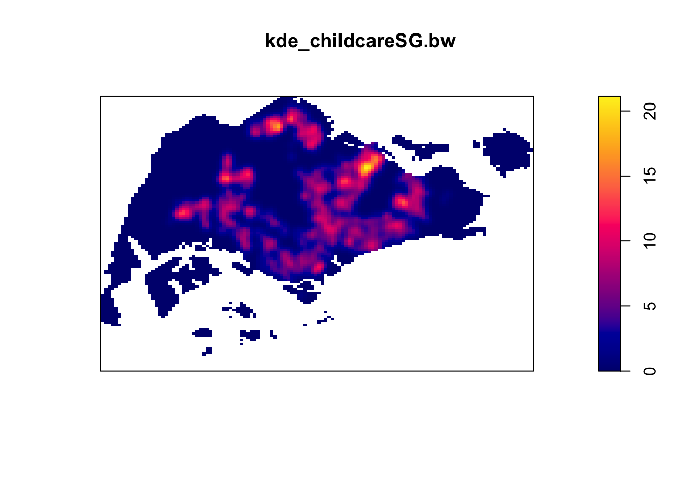
Since we just did a rescaling operation, the output image looks identical to the earlier version with the only changes in terms of data values.
11.2 Working with Different Automatic Bandwidth Methods
Beside bw.diggle(), there are 3 other
spatstat functions can be used to determine the
bandwidth, they are: bw.CvL(),
bw.scott(), and bw.ppl().
Let us take a look at the bandwidth return by these automatic bandwidth calculation methods by using:
bw.CvL(childcareSG_ppp.km) sigma
5.009037 bw.scott(childcareSG_ppp.km) sigma.x sigma.y
2.224958 1.451103 bw.ppl(childcareSG_ppp.km) sigma
0.273598 bw.diggle(childcareSG_ppp.km) sigma
0.4144576
Baddeley et al. (2016) suggest using the
bw.ppl() algorithm, as it tends to produce more
appropriate values when the pattern consists predominantly of
tight clusters. However, they also note that if the aim of a study
is to detect a single tight cluster amidst random noise, the
bw.diggle() method is likely to be more effective.
To compare the output of using bw.diggle and
bw.ppl methods:
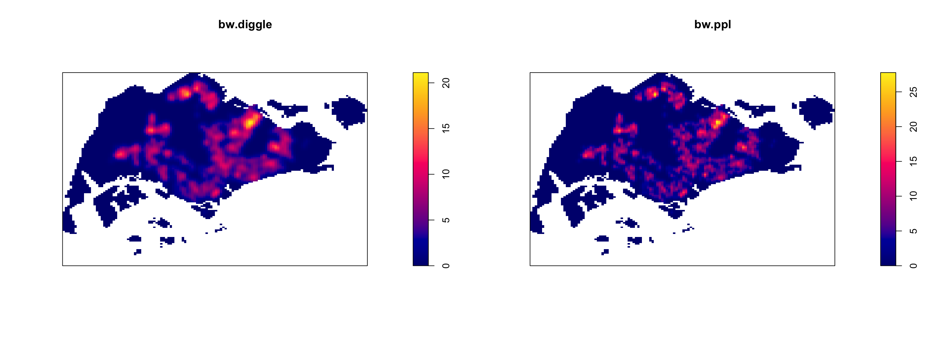
12 6.3 Working with Different Kernel Methods
By default, the kernel method used in density.ppp() is
gaussian. But there are three other options, namely:
Epanechnikov, Quartic and Dics. Let us
take a look at what they look like:
par(mfrow=c(2,2))
plot(density(childcareSG_ppp.km,
             sigma=bw.ppl,
             edge=TRUE,
             kernel="gaussian"),
     main="Gaussian")

plot(density(childcareSG_ppp.km,
             sigma=bw.ppl,
             edge=TRUE,
             kernel="epanechnikov"),
     main="Epanechnikov")

plot(density(childcareSG_ppp.km,
             sigma=bw.ppl,
             edge=TRUE,
             kernel="quartic"),
     main="Quartic")

plot(density(childcareSG_ppp.km,
             sigma=bw.ppl,
             edge=TRUE,
             kernel="disc"),
     main="Disc")
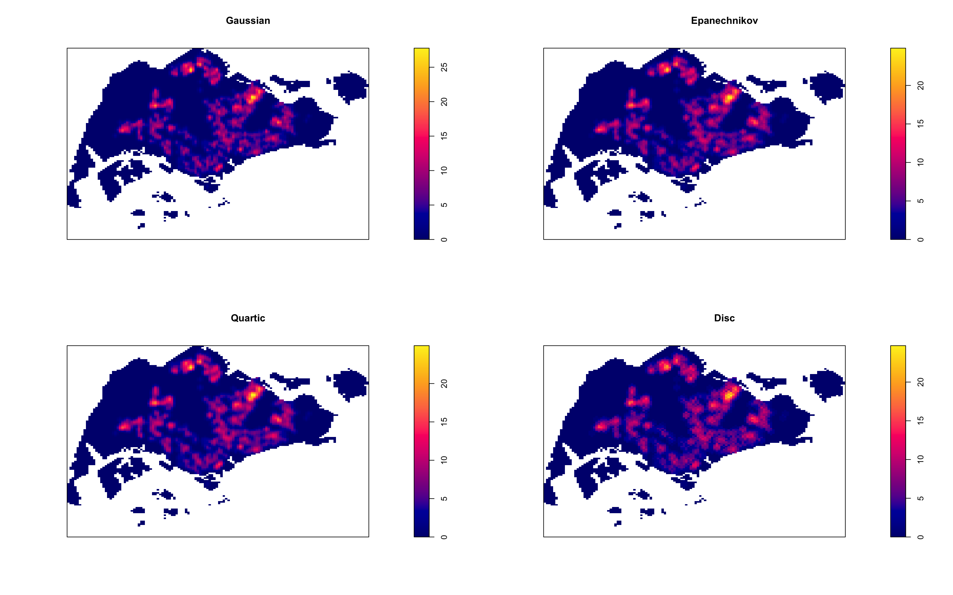
Observations: In this dataset, the choice of kernel function has only a minor impact on the overall density plots. The Gaussian, Epanechnikov, and Quartic kernels produce smoother transitions and distribute the density over a broader area. In contrast, the Disc kernel provides a more localized density estimation with sharper boundaries and less smoothness.
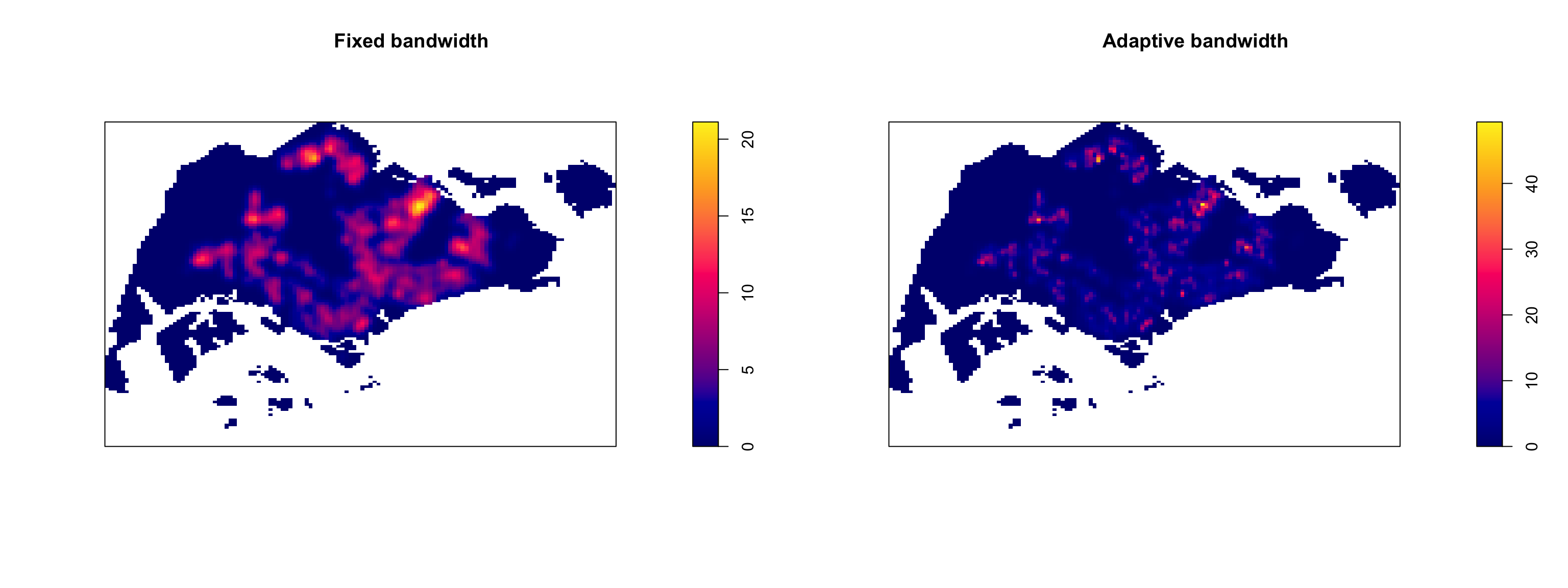
13 Fixed and Adaptive KDE
13.1 Computing KDE by using Fixed Bandwidth
Next, we will compute a KDE layer by defining a bandwidth of 600 meter. Notice that in the code block below, the sigma value used is 0.6. This is because the unit of measurement of childcareSG_ppp.km object is in kilometer, hence the 600m is 0.6km.
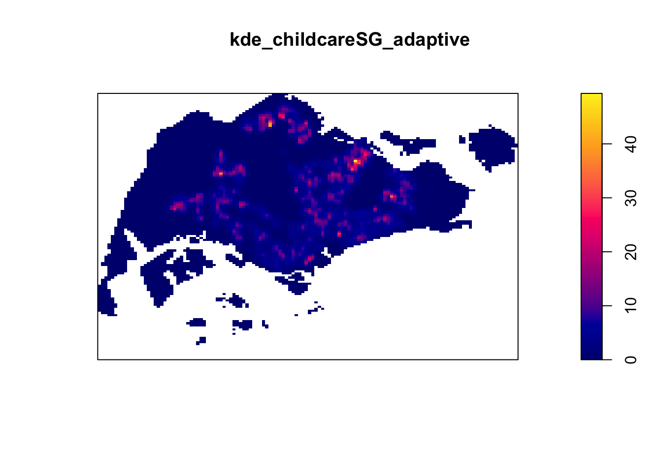
In this section, we will learn how to derive adaptive kernel
density estimation by using
density.adaptive()
of spatstat.
kde_childcareSG_adaptive <- adaptive.density(childcareSG_ppp.km, method="kernel")
plot(kde_childcareSG_adaptive)
We can compare the fixed and adaptive kernel density estimation outputs by using:
13.2 Converting KDE Output into Grid Object
To achieve the same result, we convert the object to a format suitable for mapping:
gridded_kde_childcareSG_bw <- as.SpatialGridDataFrame.im(kde_childcareSG.bw)
spplot(gridded_kde_childcareSG_bw)
13.2.1 Converting Grided Output into Raster
Next, we will convert the gridded kernel density objects into RasterLayer object by using raster() of raster package.
kde_childcareSG_bw_raster <- raster(kde_childcareSG.bw)Let us take a look at the properties of kde_childcareSG_bw_raster RasterLayer.
kde_childcareSG_bw_rasterclass : RasterLayer
dimensions : 128, 128, 16384 (nrow, ncol, ncell)
resolution : 0.4170614, 0.2647348 (x, y)
extent : 2.663926, 56.04779, 16.35798, 50.24403 (xmin, xmax, ymin, ymax)
crs : NA
source : memory
names : layer
values : -1.006362e-14, 21.11878 (min, max)Note that the crs property is NA.
13.2.2 Assigning Projection Systems
To include the CRS information on kde_childcareSG_bw_raster RasterLayer, we will do the following:
projection(kde_childcareSG_bw_raster) <- CRS("+init=EPSG:3414")
kde_childcareSG_bw_raster
class : RasterLayer
dimensions : 128, 128, 16384 (nrow, ncol, ncell)
resolution : 0.4170614, 0.2647348 (x, y)
extent : 2.663926, 56.04779, 16.35798, 50.24403 (xmin, xmax, ymin, ymax)
crs : +proj=tmerc +lat_0=1.36666666666667 +lon_0=103.833333333333 +k=1 +x_0=28001.642 +y_0=38744.572 +ellps=WGS84 +units=m +no_defs
source : memory
names : layer
values : -1.006362e-14, 21.11878 (min, max)Now, the crs property is completed.
13.3 Visualising the output in tmap
Finally, we will display the raster in cartographic quality map
using tmap package.
tm_shape(kde_childcareSG_bw_raster) +
  tm_raster("layer", palette = "viridis") +
  tm_layout(legend.position = c("right", "bottom"), frame = FALSE)
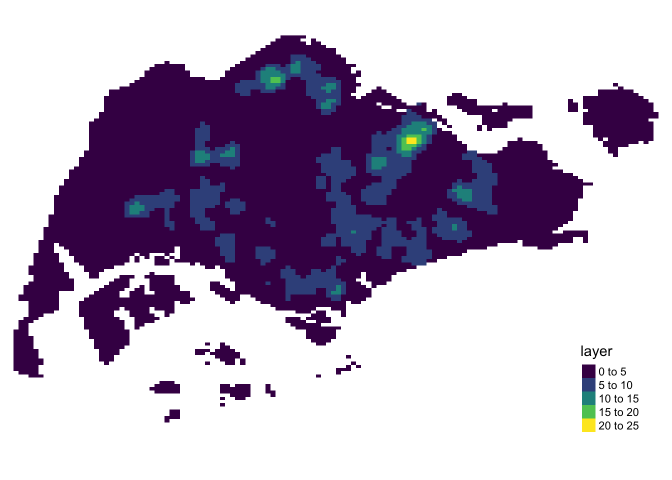
values(kde_childcareSG_bw_raster)Note that the raster values are encoded explicitly onto the raster pixel using the values in “v” field.
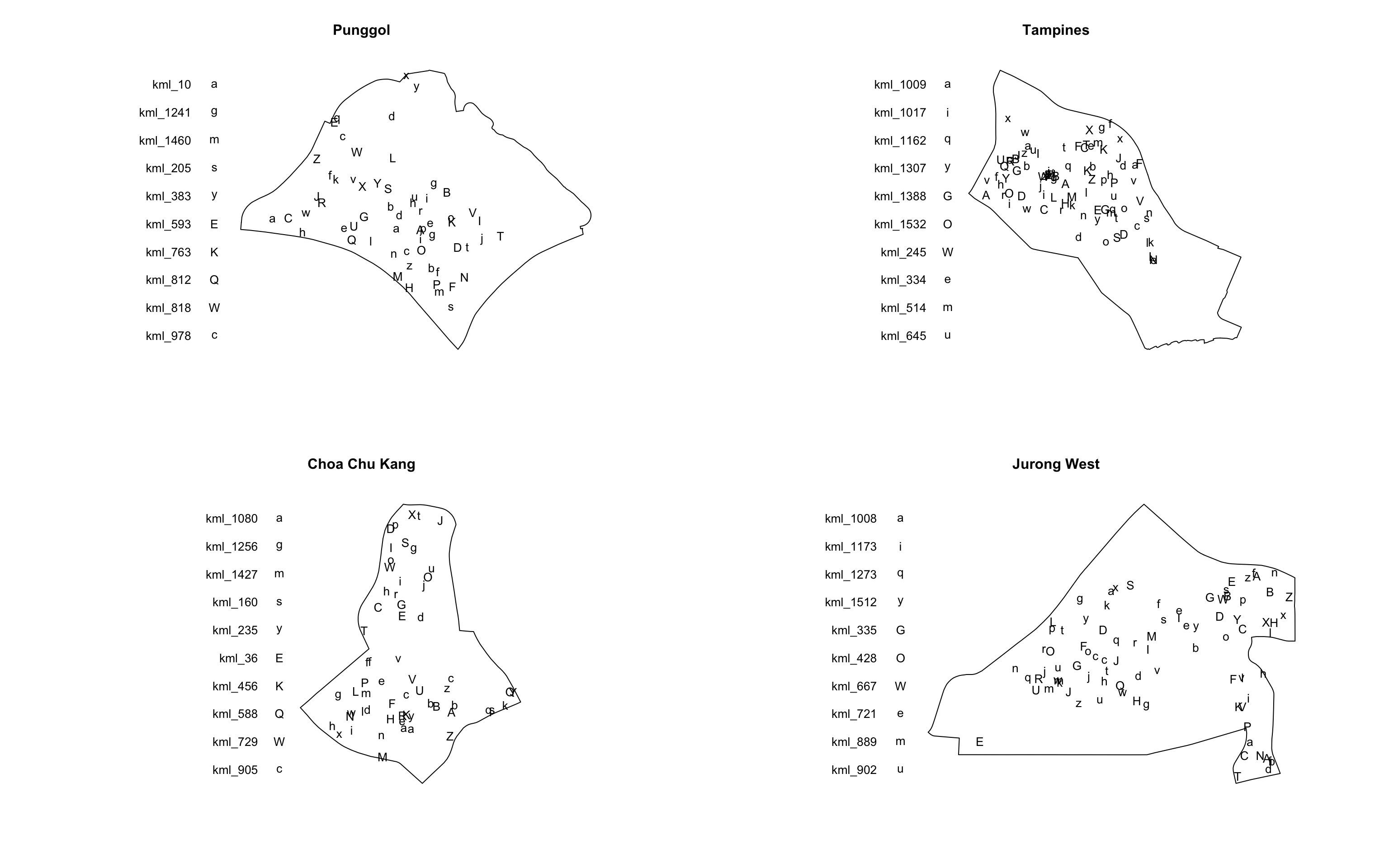
13.4 Comparing Spatial Point Patterns using KDE
In this section, we will learn how to compare KDE of childcare at Punggol, Tampines, Chua Chu Kang and Jurong West planning areas.
13.4.1 Extracting Study Area
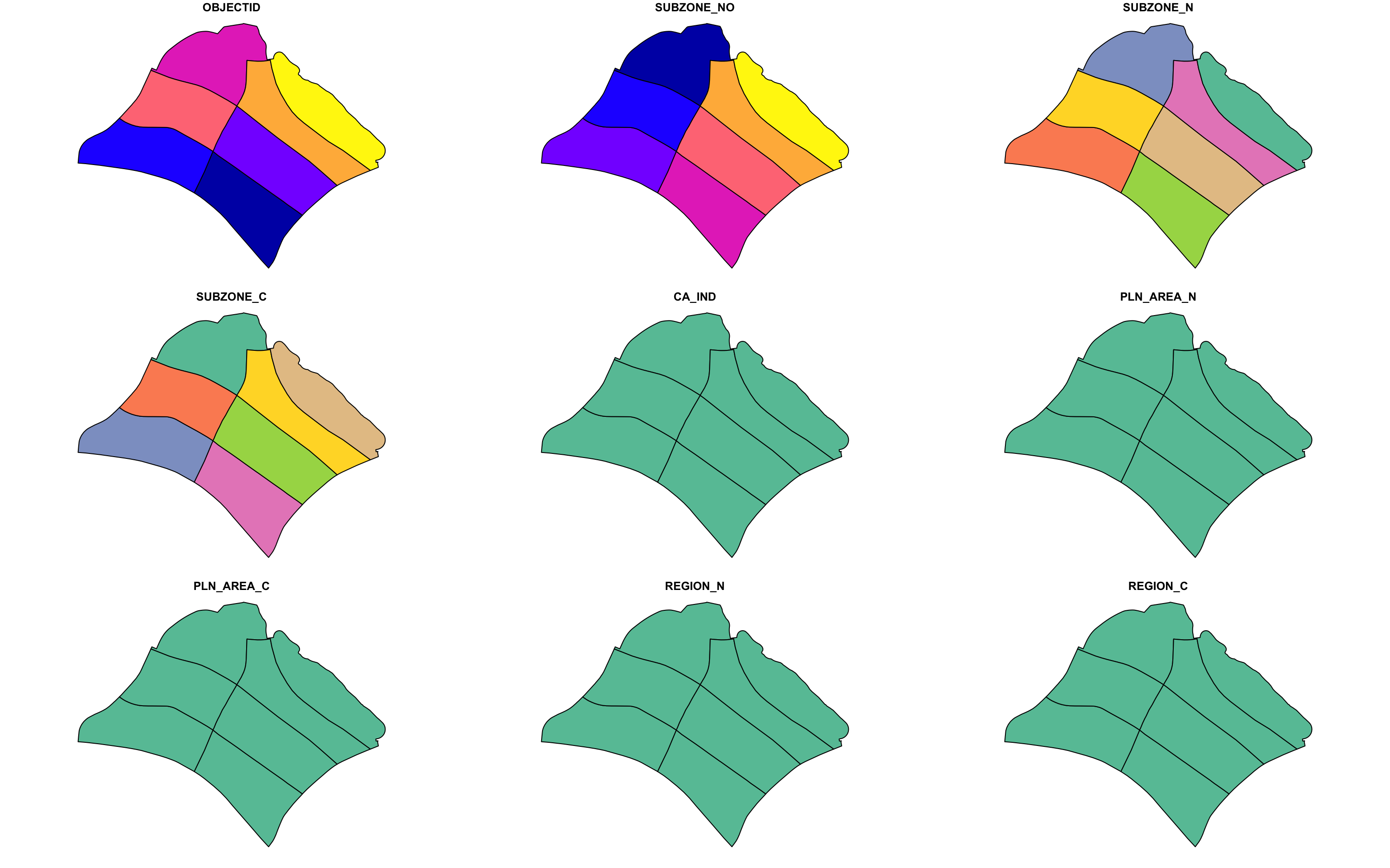
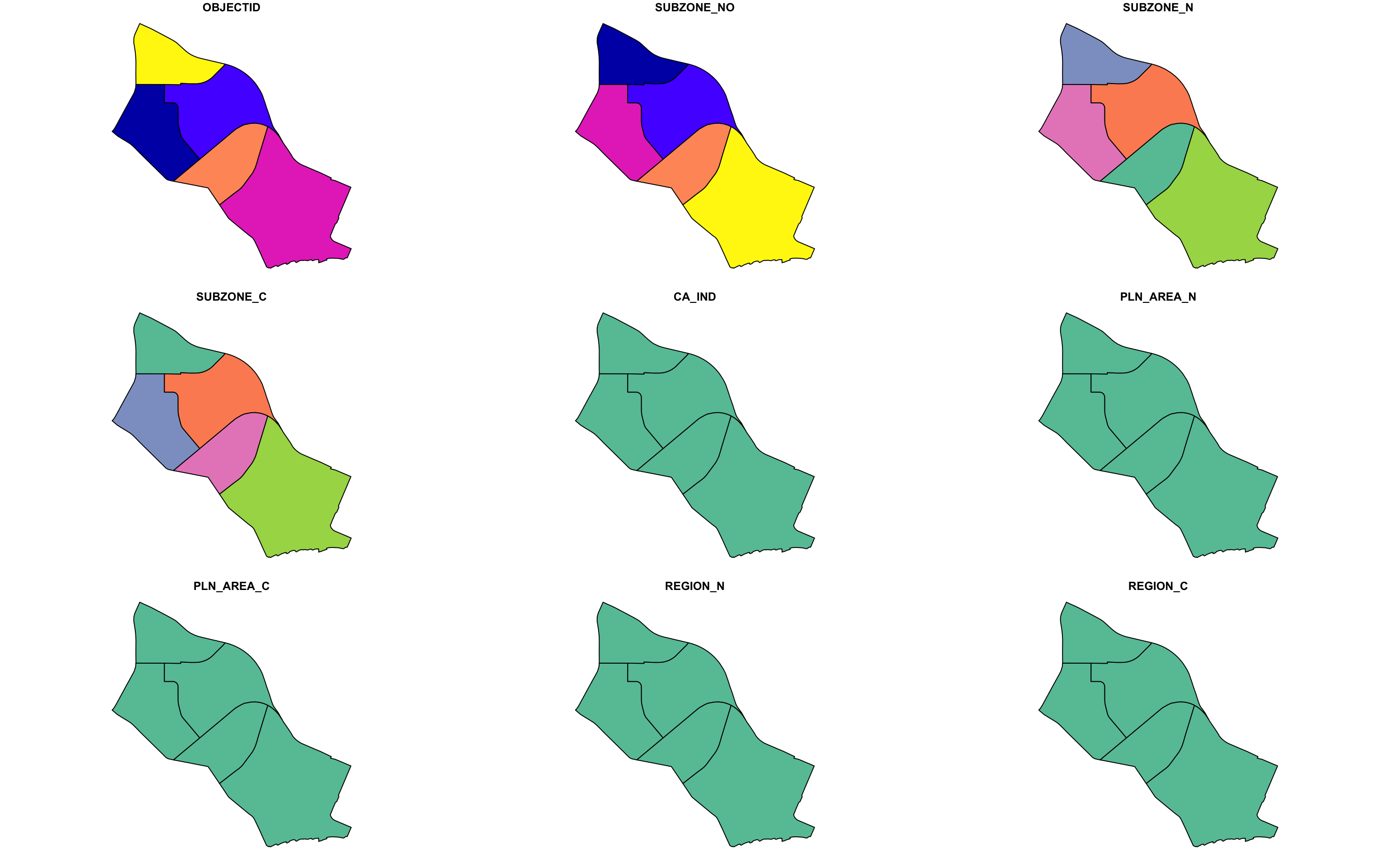
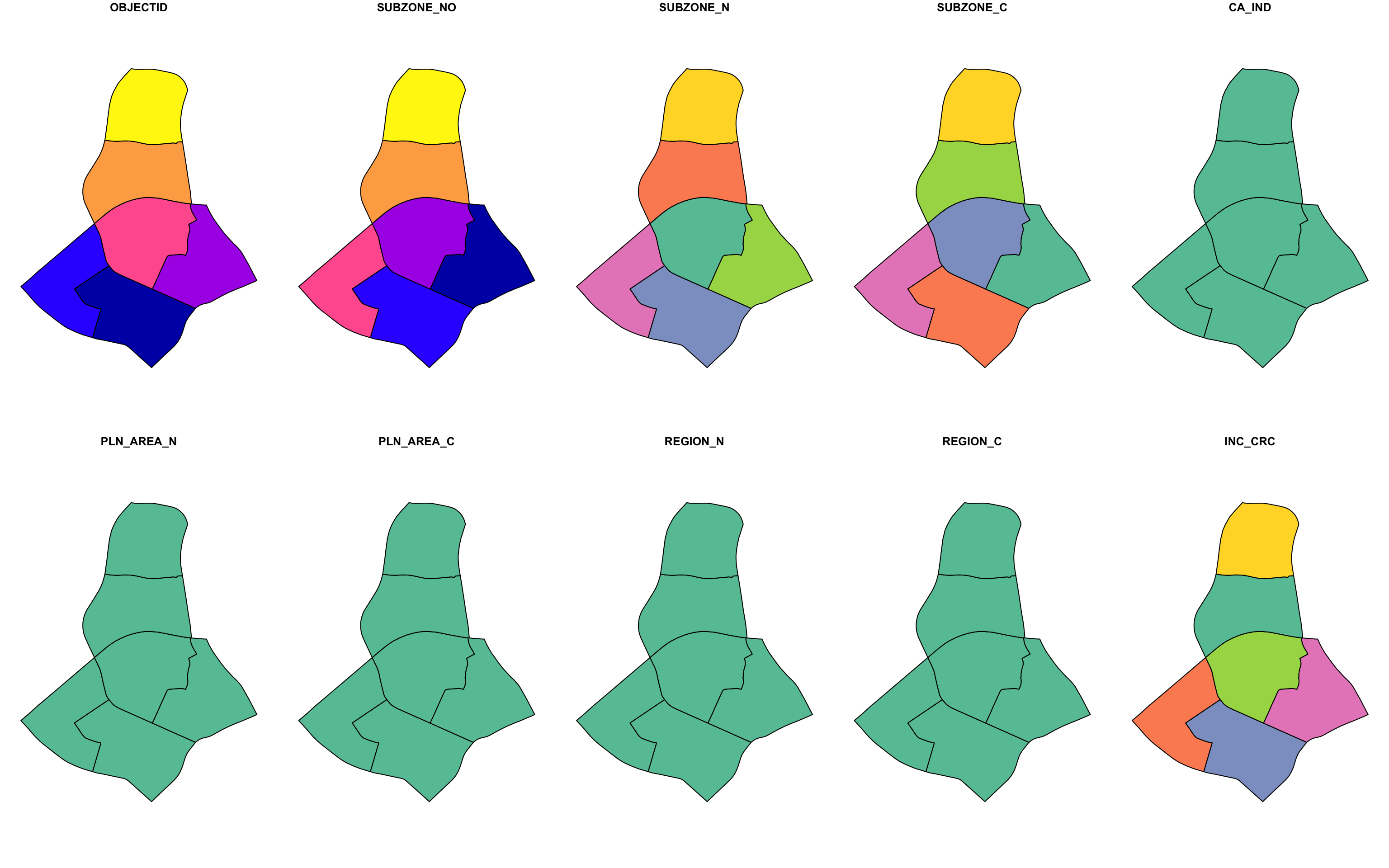
The code block below will be used to extract the target planning areas.
Plotting the target planning areas:
13.4.2 Creating owin object
Now, we will convert these sf objects into owin objects that is required by spatstat.
pg_owin = as.owin(pg)
tm_owin = as.owin(tm)
ck_owin = as.owin(ck)
jw_owin = as.owin(jw)
13.4.3 Combining Childcare Points and the Study Area
To extract childcare that is within the specific region for analysis, we can use:
childcare_pg_ppp = childcare_ppp_jit[pg_owin]
childcare_tm_ppp = childcare_ppp_jit[tm_owin]
childcare_ck_ppp = childcare_ppp_jit[ck_owin]
childcare_jw_ppp = childcare_ppp_jit[jw_owin]
Next, rescale.ppp() function is used to transform
the unit of measurement from meter to kilometer.
childcare_pg_ppp.km = rescale.ppp(childcare_pg_ppp, 1000, "km")
childcare_tm_ppp.km = rescale.ppp(childcare_tm_ppp, 1000, "km")
childcare_ck_ppp.km = rescale.ppp(childcare_ck_ppp, 1000, "km")
childcare_jw_ppp.km = rescale.ppp(childcare_jw_ppp, 1000, "km")
The code block below is used to plot the four study areas and the locations of the childcare centres.
14 Second-Order Spatial Point Pattern Analysis
In this section, we will analyze spatial point patterns using various functions: G-Function, F-Function, K-Function, and L-Function.
14.1 Analysing Spatial Point Process Using G-Function
The G function measures the distribution of the distances from an
arbitrary event to its nearest event. In this section, we will
learn how to compute G-function estimation by using
Gest()
of spatstat package. We will also learn how to
perform monte carlo simulation test using
envelope()
of spatstat package.
14.1.1 Choa Chu Kang Planning Area
14.1.1.1 Computing G-function Estimation
To compute G-function using Gest() of
spatstat package:
Note
correction is an optional argument in
Gest()
Optional. The edge correction(s) to be used to estimate . A vector of character strings selected from “none”, “rs”, “km”, “Hanisch” and “best”. Alternatively correction=“all” selects all options.
# rs and border has the same effect
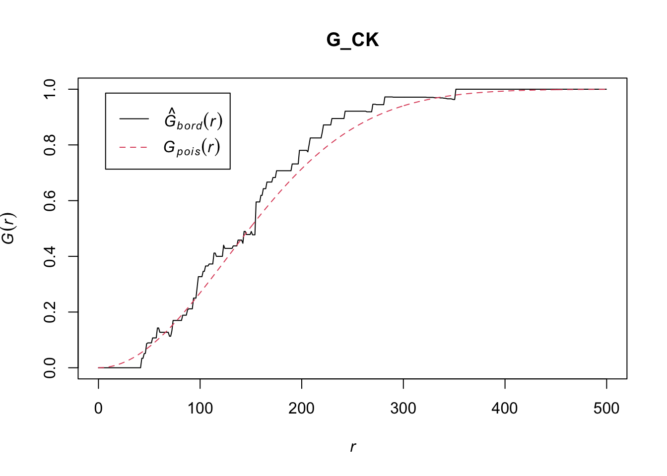
G_CK = Gest(childcare_ck_ppp, correction = "rs")
G_CK = Gest(childcare_ck_ppp, correction = "border")
plot(G_CK, xlim=c(0,500))
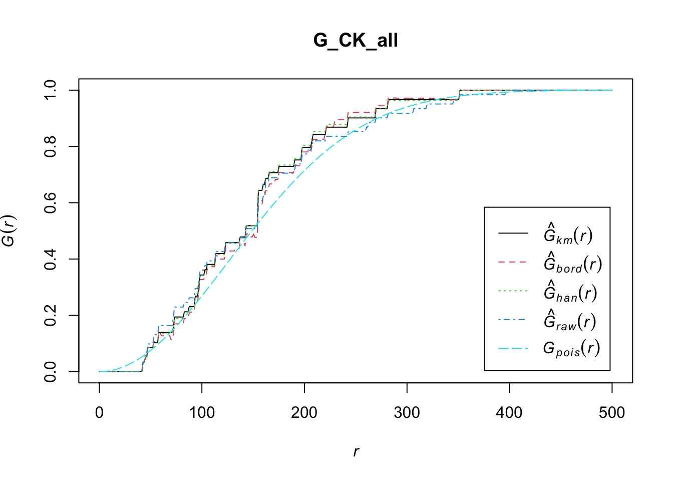
We can also use the “all” option in correction to display all forms of edge corrections from “none”, “rs”, “km”, “Hanisch” and “best”.
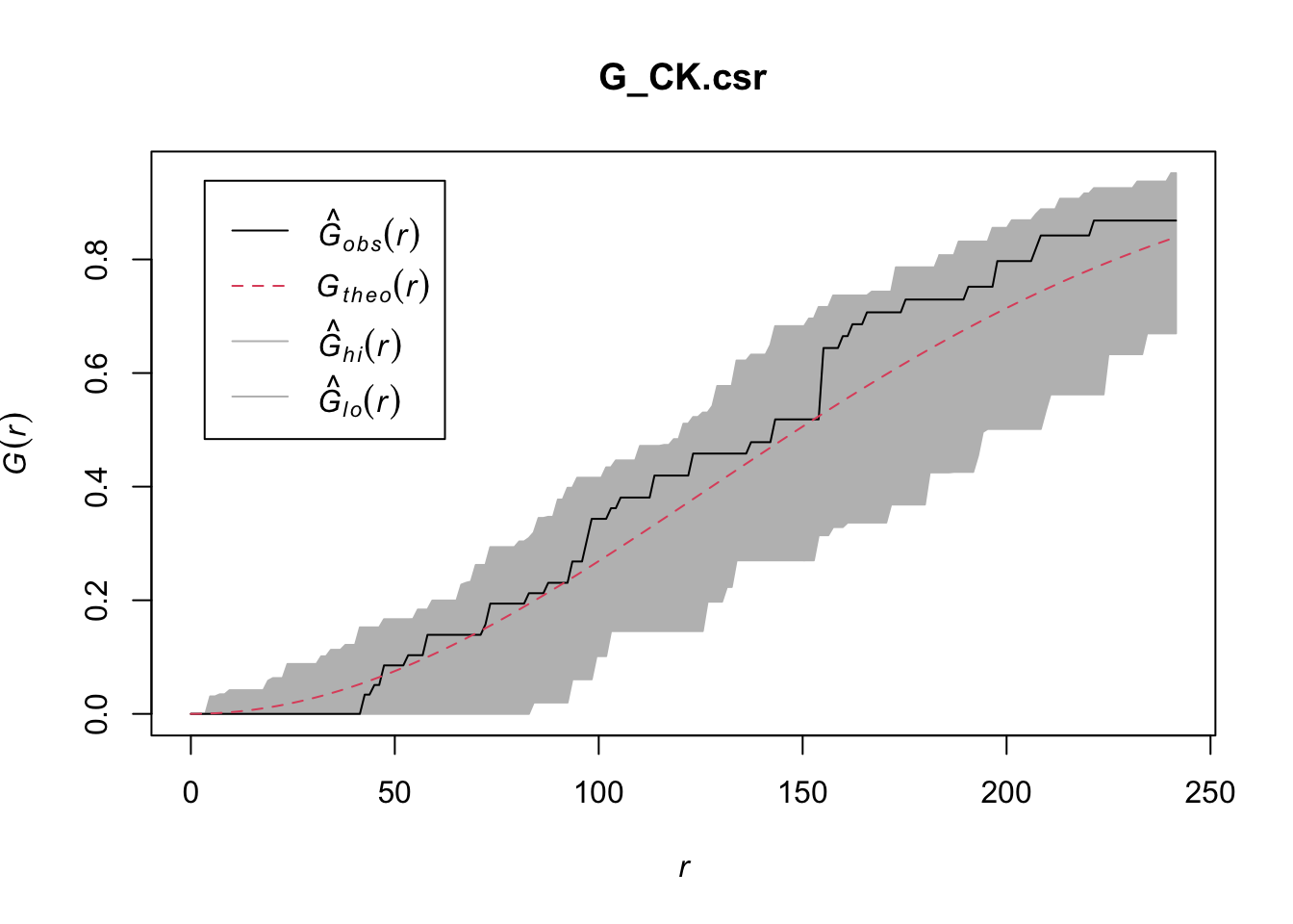
14.1.1.2 Performing Complete Spatial Randomness Test
To confirm the observed spatial patterns above, a hypothesis test will be conducted. The hypothesis and test are as follows:
\(H_0\) = The distribution of childcare services at Choa Chu Kang are randomly distributed.
\(H_1\)= The distribution of childcare services at Choa Chu Kang are not randomly distributed.
The null hypothesis will be rejected if p-value is smaller than alpha value of 0.001.
Monte Carlo test with G-function:
Note
The envelope function calculates overall and pointwise confidence envelopes for a curve based on bootstrap replicates of the curve evaluated at a number of fixed points.
In other words, It helps you determine if your observed spatial pattern (e.g., locations of points in a study area) is significantly different from what you would expect under a random or theoretical distribution.
How It Works: 1. Simulate Data: It generates multiple simulated datasets (often by randomizing the locations of points) based on the null hypothesis (e.g., complete spatial randomness). 2. Compute Statistics: For each simulated dataset, it computes a spatial statistic (e.g., G-function, F-function) and creates a distribution of these statistics. 3. Compare: It compares the observed statistic from your actual data to the distribution of statistics from the simulated datasets. 4. Envelope Plot: It plots the range (envelope) of the simulated statistics along with the observed statistic, allowing you to see if your observed statistic falls outside the range of what is expected under the null hypothesis.
When to Use It? Use the envelope function when you want to:
- Test if the observed spatial pattern deviates significantly from a random pattern or other theoretical patterns.
- Assess the statistical significance of spatial features or clustering in your data.
Choice of nsim: The choice
of 39 simulations (nsim = 39) in Monte Carlo techniques
for spatial analysis is often a practical compromise
between computational efficiency and statistical
robustness.
- Computational Efficiency: Running a large number of simulations can be computationally expensive, especially for complex spatial analyses. We can strike a balance between obtaining reliable results and keeping computational costs manageable by selecting absolute minimum sample size.
The minimum number of simulations \(m\) required for a Monte Carlo test at a particular significance level can be determined by:
\(\alpha = \frac{1}{m+1}\)
for a one-tailed test and
\(\alpha = \frac{2}{m+1}\)
Thus, a one-tailed test at a significance level of 5% would require a minimum of 19 simulations, a two-tailed test at a significance level of 5% would require a minimum of 39 simulations.
see Going beyond the required number of simulations required for a particular significance level when conducting a Monte Carlo test - Cross Validated, spatial statistics - Simulation envelopes and significance levels - Geographic Information Systems Stack Exchange
G_CK.csr <- envelope(childcare_ck_ppp, Gest, nsim=39)Generating 39 simulations of CSR ...
1, 2, 3, 4, 5, 6, 7, 8, 9, 10, 11, 12, 13, 14, 15, 16, 17, 18, 19, 20,
21, 22, 23, 24, 25, 26, 27, 28, 29, 30, 31, 32, 33, 34, 35, 36, 37, 38,
39.
Done.plot(G_CK.csr)
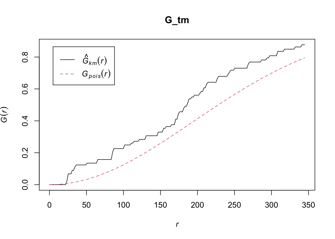
14.1.2 Tampines Planning Area
14.1.2.1 Computing G-function Estimation
We will use the best edge correction for this
example.
G_tm = Gest(childcare_tm_ppp, correction = "best")
plot(G_tm)
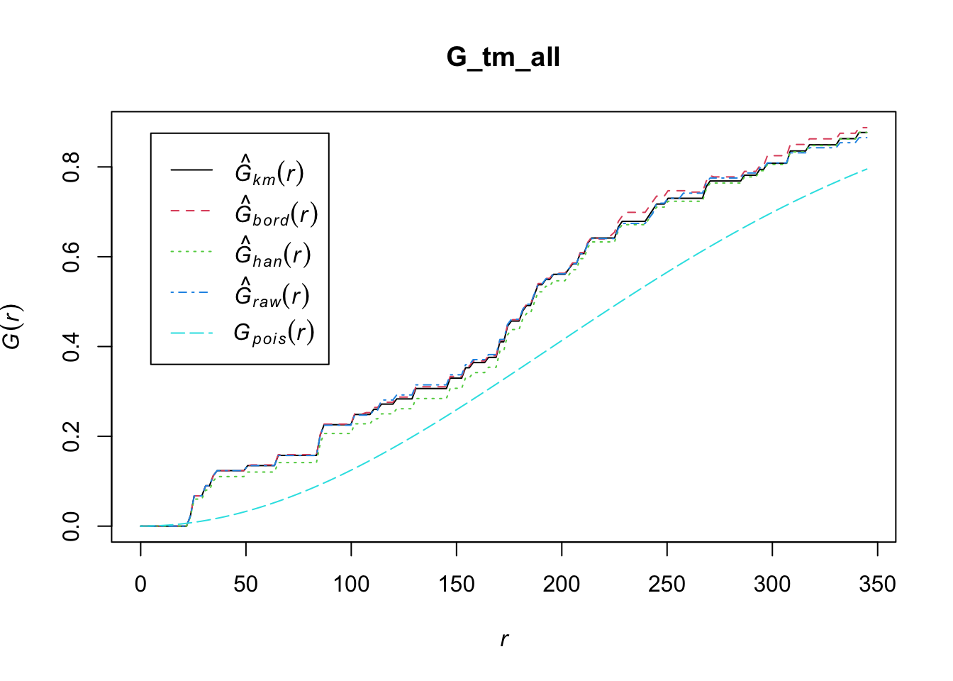
G_tm_all = Gest(childcare_tm_ppp, correction = "all")
plot(G_tm_all)
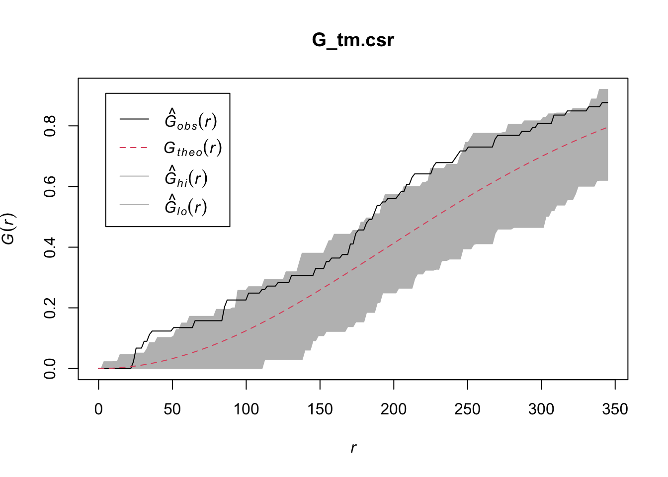
14.2 Performing Complete Spatial Randomness Test
To confirm the observed spatial patterns above, a hypothesis test will be conducted. The hypothesis and test are as follows:
\(H_0\) = The distribution of childcare services at Tampines are randomly distributed.
\(H_1\) = The distribution of childcare services at Tampines are not randomly distributed.
The null hypothesis will be rejected is p-value is smaller than alpha value of 0.001.
The code block below is used to perform the hypothesis testing.
G_tm.csr <- envelope(childcare_tm_ppp, Gest, correction = "all", nsim=39)Generating 39 simulations of CSR ...
1, 2, 3, 4, 5, 6, 7, 8, 9, 10, 11, 12, 13, 14, 15, 16, 17, 18, 19, 20,
21, 22, 23, 24, 25, 26, 27, 28, 29, 30, 31, 32, 33, 34, 35, 36, 37, 38,
39.
Done.plot(G_tm.csr)
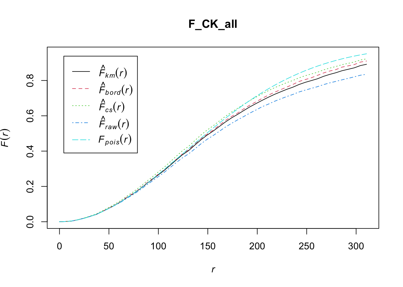
14.3 Analysing Spatial Point Process Using F-Function
The F function estimates the empty space function F(r) or its
hazard rate h(r) from a point pattern in a window of arbitrary
shape. In this section, we will learn how to compute F-function
estimation by using
Fest()
of spatstat package. We will also learn how to
perform monte carlo simulation test using
envelope()
of spatstat package.
14.3.1 Choa Chu Kang Planning Area
14.3.1.1 Computing F-function estimation
Note
Fest() has the same correction option as
Gest().
F_CK_all = Fest(childcare_ck_ppp, correction = "all")
plot(F_CK_all)
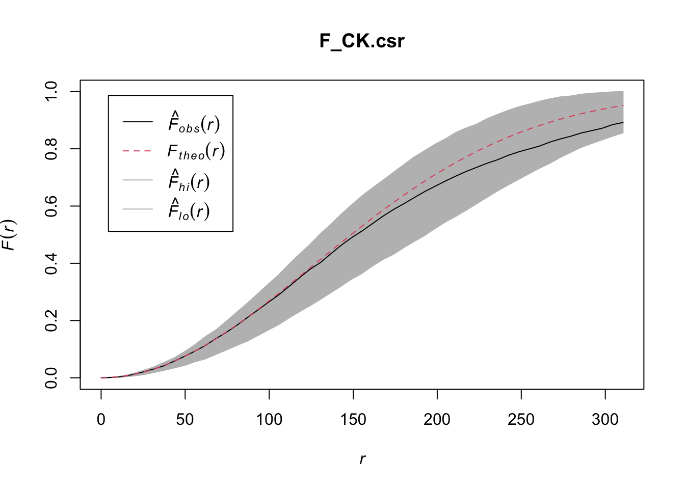
14.3.1.2 Performing Complete Spatial Randomness Test
To confirm the observed spatial patterns above, a hypothesis test will be conducted. The hypothesis and test are as follows:
\(H_0\) = The distribution of childcare services at Choa Chu Kang are randomly distributed.
\(H_1\) = The distribution of childcare services at Choa Chu Kang are not randomly distributed.
The null hypothesis will be rejected if p-value is smaller than alpha value of 0.001.
Monte Carlo test with F-function:
F_CK.csr <- envelope(childcare_ck_ppp, Fest, nsim=39)Generating 39 simulations of CSR ...
1, 2, 3, 4, 5, 6, 7, 8, 9, 10, 11, 12, 13, 14, 15, 16, 17, 18, 19, 20,
21, 22, 23, 24, 25, 26, 27, 28, 29, 30, 31, 32, 33, 34, 35, 36, 37, 38,
39.
Done.plot(F_CK.csr)
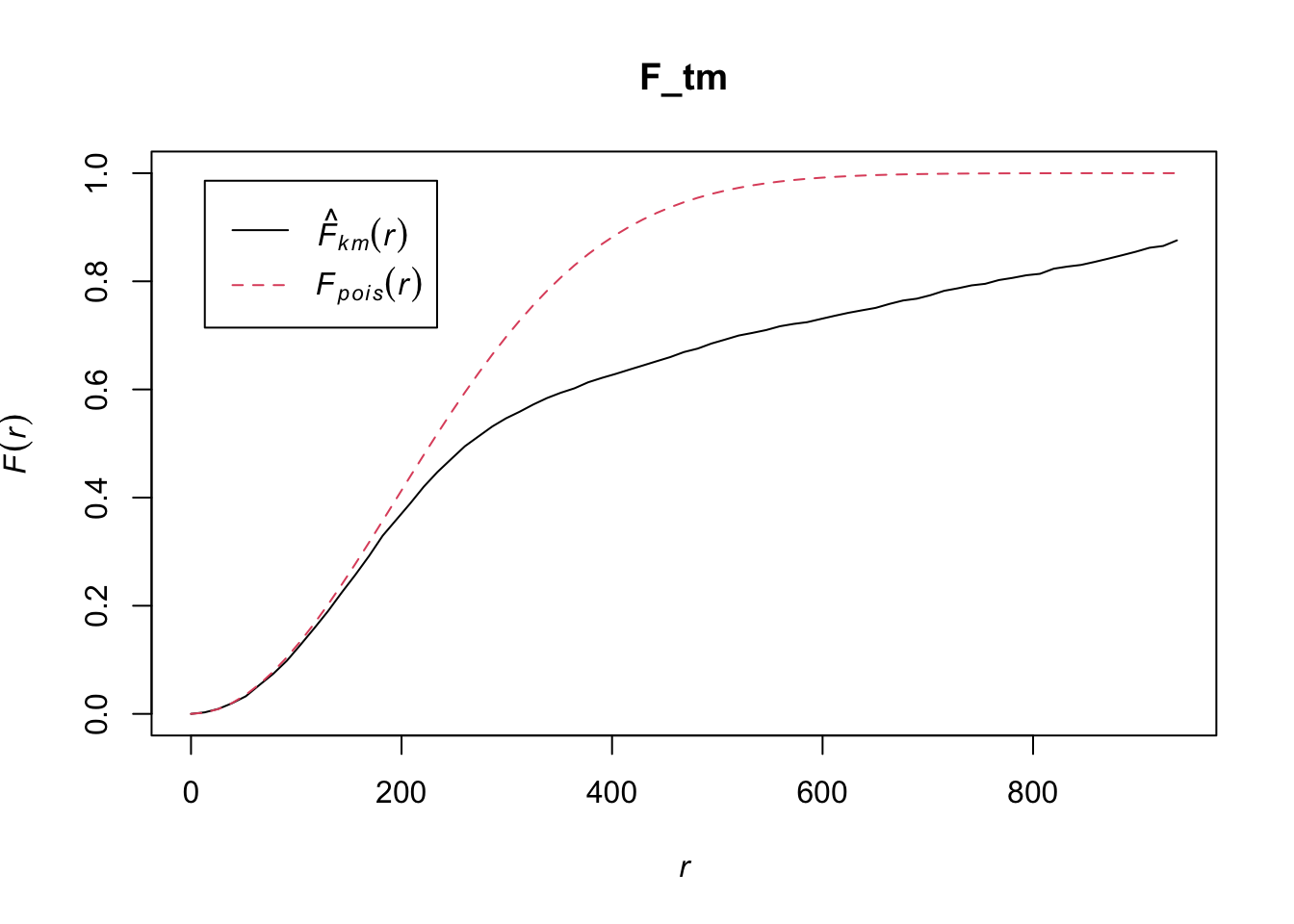
14.3.2 Tampines Planning Area
14.3.2.1 Computing F-function estimation
Monte Carlo test with F-function:
F_tm = Fest(childcare_tm_ppp, correction = "best")
plot(F_tm)
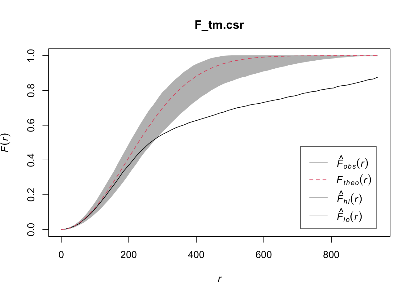
14.3.2.2 Performing Complete Spatial Randomness Test
To confirm the observed spatial patterns above, a hypothesis test will be conducted. The hypothesis and test are as follows:
\(H_0\) = The distribution of childcare services at Tampines are randomly distributed.
\(H_1\) = The distribution of childcare services at Tampines are not randomly distributed.
The null hypothesis will be rejected is p-value is smaller than alpha value of 0.001.
The code block below is used to perform the hypothesis testing.
F_tm.csr <- envelope(childcare_tm_ppp, Fest, correction = "all", nsim=39)Generating 39 simulations of CSR ...
1, 2, 3, 4, 5, 6, 7, 8, 9, 10, 11, 12, 13, 14, 15, 16, 17, 18, 19, 20,
21, 22, 23, 24, 25, 26, 27, 28, 29, 30, 31, 32, 33, 34, 35, 36, 37, 38,
39.
Done.plot(F_tm.csr)
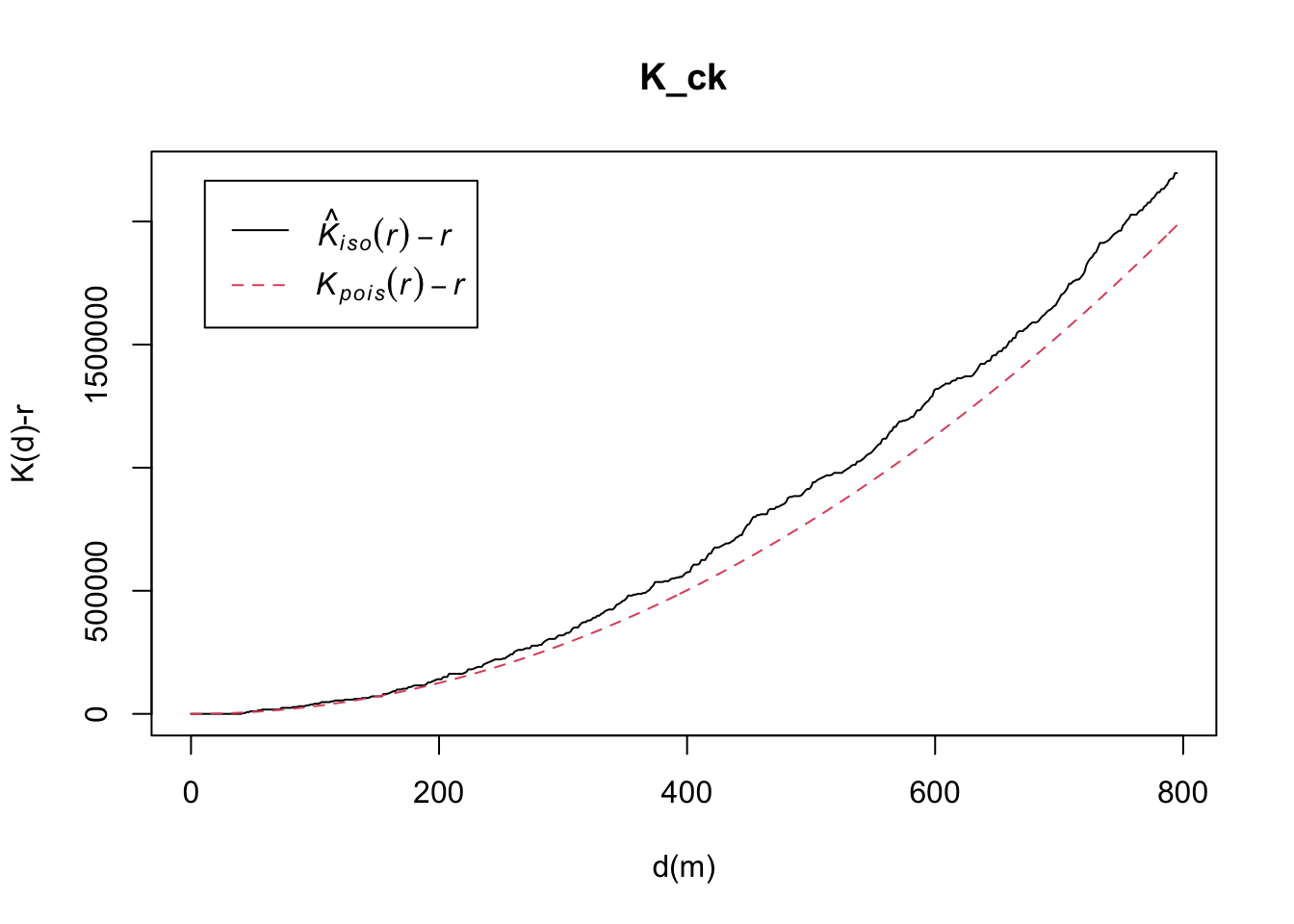
14.4 Analysing Spatial Point Process Using K-Function
K-function measures the number of events found up to a given
distance of any particular event. In this section, you will learn
how to compute K-function estimates by using
Kest()
of spatstat package. We will also learn how to
perform monte carlo simulation test using
envelope()
of spatstat package.
Note
Kest()’s
correction option is different fromGest()andFest()`.
correction: Optional. A character vector
containing any selection of the options “none”, “border”,
“bord.modif”, “isotropic”, “Ripley”, “translate”,
“translation”, “rigid”, “none”, “good” or “best”. It specifies
the edge correction(s) to be applied. Alternatively
correction=“all” selects all options.
14.4.1 Choa Chu Kang Planning Area
14.4.1.1 Computing K-Function Estimate
K_ck = Kest(childcare_ck_ppp, correction = "Ripley")
plot(K_ck, . -r ~ r, ylab= "K(d)-r", xlab = "d(m)")
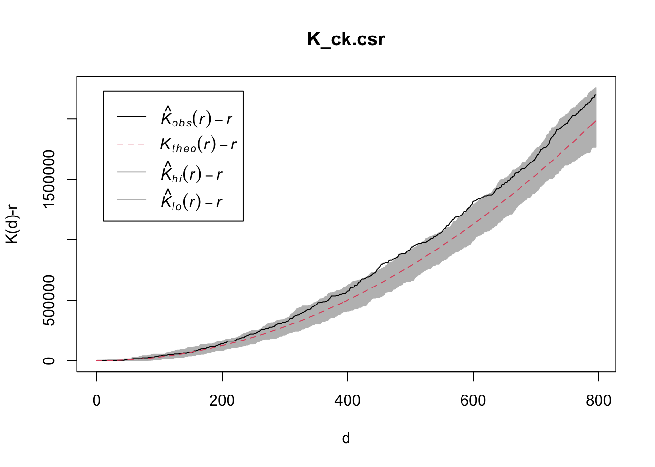
14.4.1.2 Performing Complete Spatial Randomness Test
To confirm the observed spatial patterns above, a hypothesis test will be conducted. The hypothesis and test are as follows:
\(H_0\) = The distribution of childcare services at Choa Chu Kang are randomly distributed.
\(H_1\) = The distribution of childcare services at Choa Chu Kang are not randomly distributed.
The null hypothesis will be rejected if p-value is smaller than alpha value of 0.001.
The code block below is used to perform the hypothesis testing.
K_ck.csr <- envelope(childcare_ck_ppp, Kest, nsim=39, rank = 1, glocal=TRUE)Generating 39 simulations of CSR ...
1, 2, 3, 4, 5, 6, 7, 8, 9, 10, 11, 12, 13, 14, 15, 16, 17, 18, 19, 20,
21, 22, 23, 24, 25, 26, 27, 28, 29, 30, 31, 32, 33, 34, 35, 36, 37, 38,
39.
Done.plot(K_ck.csr, . - r ~ r, xlab="d", ylab="K(d)-r")
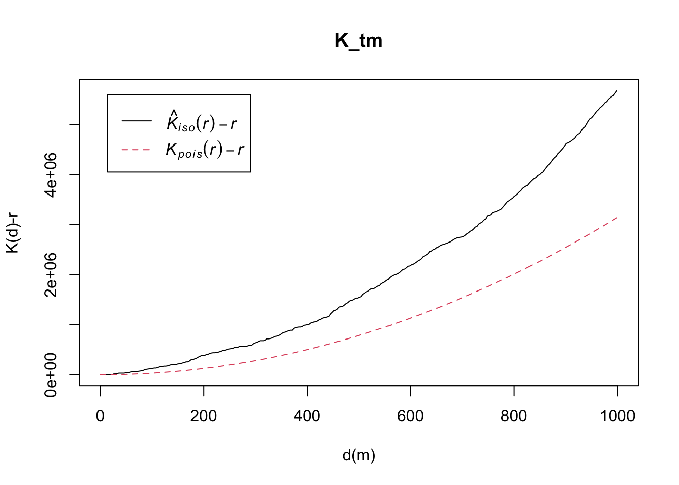
14.4.2 Tampines Planning Area
14.4.2.1 Computing K-function Estimation
14.5 Performing Complete Spatial Randomness Test
To confirm the observed spatial patterns above, a hypothesis test will be conducted. The hypothesis and test are as follows:
\(H_0\) = The distribution of childcare services at Tampines are randomly distributed.
\(H_1\) = The distribution of childcare services at Tampines are not randomly distributed.
The null hypothesis will be rejected if p-value is smaller than alpha value of 0.001.
The code block below is used to perform the hypothesis testing.
K_tm.csr <- envelope(childcare_tm_ppp, Kest, nsim=39, rank = 1, glocal=TRUE)Generating 39 simulations of CSR ...
1, 2, 3, 4, 5, 6, 7, 8, 9, 10, 11, 12, 13, 14, 15, 16, 17, 18, 19, 20,
21, 22, 23, 24, 25, 26, 27, 28, 29, 30, 31, 32, 33, 34, 35, 36, 37, 38,
39.
Done.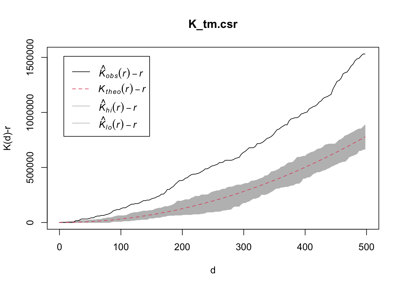
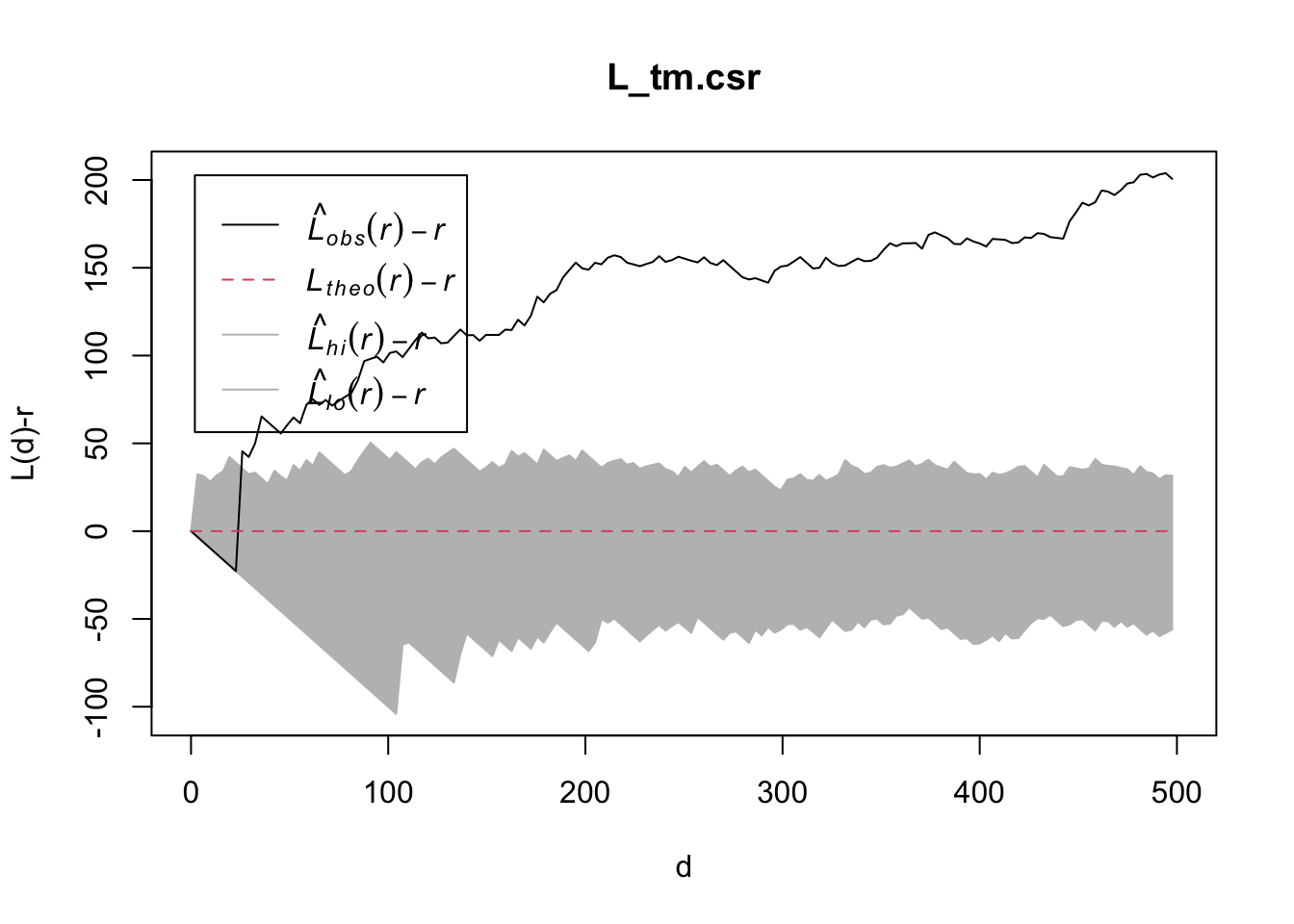
14.6 Analysing Spatial Point Process Using L-Function
In this section, you will learn how to compute L-function
estimation by using
Lest()
of spatstat package. We will also learn how to
perform monte carlo simulation test using
envelope()
of spatstat package.
14.6.1 Choa Chu Kang Planning Area
14.6.1.1 Computing L-function Estimation
Note
Lest() has the same correction options as
Kest().
L_ck = Lest(childcare_ck_ppp, correction = "Ripley")
plot(L_ck, . -r ~ r,
     ylab= "L(d)-r", xlab = "d(m)")
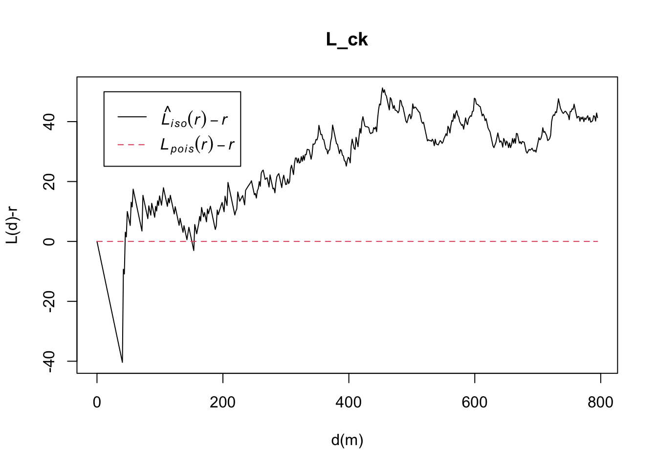
14.6.1.2 Performing Complete Spatial Randomness Test
\(H_0\) = The distribution of childcare services at Choa Chu Kang are randomly distributed.
\(H_1\) = The distribution of childcare services at Choa Chu Kang are not randomly distributed.
The null hypothesis will be rejected if p-value if smaller than alpha value of 0.001.
The code block below is used to perform the hypothesis testing.
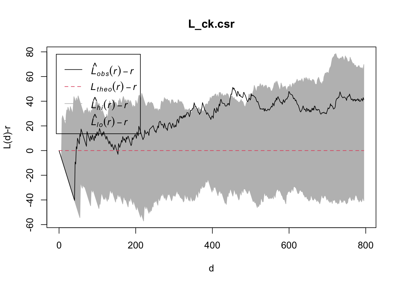
L_ck.csr <- envelope(childcare_ck_ppp, Lest, nsim=39, rank = 1, glocal=TRUE)Generating 39 simulations of CSR ...
1, 2, 3, 4, 5, 6, 7, 8, 9, 10, 11, 12, 13, 14, 15, 16, 17, 18, 19, 20,
21, 22, 23, 24, 25, 26, 27, 28, 29, 30, 31, 32, 33, 34, 35, 36, 37, 38,
39.
Done.plot(L_ck.csr, . - r ~ r, xlab="d", ylab="L(d)-r")
14.6.2 Tampines Planning Area
14.6.2.1 Computing L-function Estimate
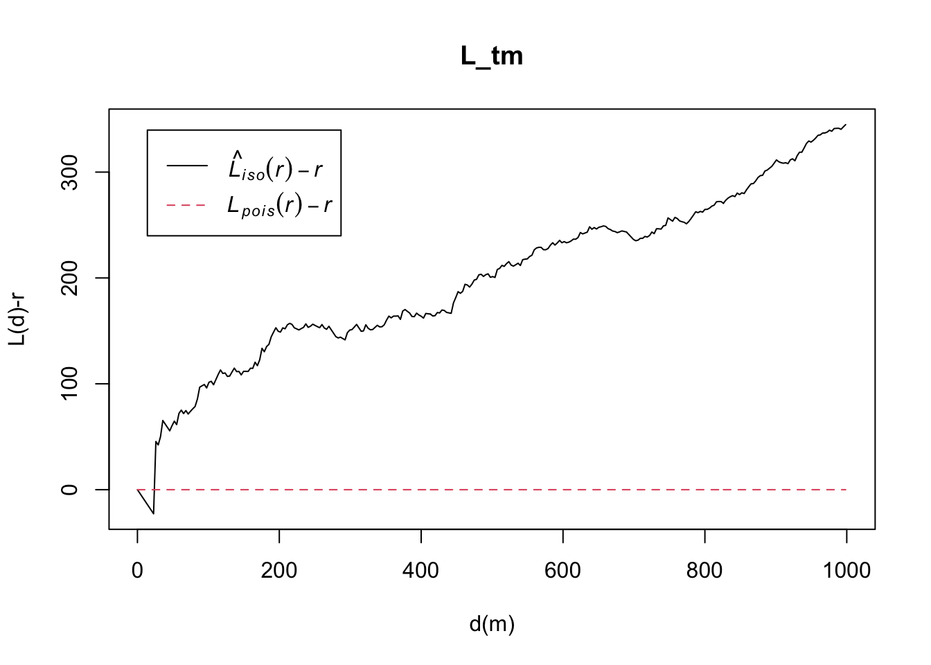
14.7 Performing Complete Spatial Randomness Test
To confirm the observed spatial patterns above, a hypothesis test will be conducted. The hypothesis and test are as follows:
\(H_0\) = The distribution of childcare services at Tampines are randomly distributed.
\(H_1\) = The distribution of childcare services at Tampines are not randomly distributed.
The null hypothesis will be rejected if p-value is smaller than alpha value of 0.001.
The code chunk below will be used to perform the hypothesis testing
L_tm.csr <- envelope(childcare_tm_ppp, Lest, nsim=39, rank = 1, glocal=TRUE)Generating 39 simulations of CSR ...
1, 2, 3, 4, 5, 6, 7, 8, 9, 10, 11, 12, 13, 14, 15, 16, 17, 18, 19, 20,
21, 22, 23, 24, 25, 26, 27, 28, 29, 30, 31, 32, 33, 34, 35, 36, 37, 38,
39.
Done.