pacman::p_load(olsrr, corrplot, ggpubr, sf, spdep, GWmodel, tmap, tidyverse, gtsummary)7A: Calibrating Hedonic Pricing Model for Private Highrise Property with GWR Method
In this exercise, we will learn to build hedonic pricing models for private high-rise property using Geographically Weighted Regression (GWR) methods to account for non-stationary variables.
1 Exercise 7A Reference
2 Overview
In this exercise, we will learn to build hedonic pricing models for private high-rise property using Geographically Weighted Regression (GWR) methods to account for non-stationary variables.
Geographically weighted regression (GWR) is a spatial statistical technique that takes non-stationary variables into consideration (e.g., climate; demographic factors; physical environment characteristics) and models the local relationships between these independent variables and an outcome of interest (also known as dependent variable).
In this exercise, The dependent variable is the resale prices of condominium in 2015. The independent variables are divided into either structural and locational.
We will be using the GWmodel package. It provides a collection of localised spatial statistical methods, namely: GW summary statistics, GW principal components analysis, GW discriminant analysis and various forms of GW regression; some of which are provided in basic and robust (outlier resistant) forms. Commonly, outputs or parameters of the GWmodel are mapped to provide a useful exploratory tool, which can often precede (and direct) a more traditional or sophisticated statistical analysis.
3 Learning Outcome
- Understand the basics of geographically weighted regression (GWR).
- Build and evaluate hedonic pricing models using GWR.
- Convert geospatial and aspatial data into appropriate formats for analysis.
- Perform exploratory data analysis (EDA) using statistical graphics.
- Visualize the model outputs and spatial patterns using various R packages.
- Assess spatial autocorrelation and other statistical properties of model residuals.
- Compare and interpret fixed and adaptive bandwidth GWR models.
4 The Data
The following 2 datasets will be used in this study:
| Data Set | Description | Format |
|---|---|---|
| MP14_SUBZONE_WEB_PL | URA Master Plan 2014’s planning subzone boundaries represented as polygon features. | ESRI Shapefile |
| condo_resale_2015.csv | Data on condominium resale prices in 2015, including structural and locational attributes. | CSV |
5 Installing and Launching the R Packages
The following R packages will be used in this exercise:
| Package | Purpose | Use Case in Exercise |
|---|---|---|
| sf | Manages, processes, and manipulates vector-based geospatial data. | Handling and converting geospatial data such as the URA Master Plan boundaries. |
| GWmodel | Calibrates geographically weighted models for local spatial analysis. | Building hedonic pricing models using fixed and adaptive bandwidth GWR methods. |
| olsrr | Performs diagnostics and builds better multiple linear regression models. | Testing for multicollinearity, normality, and linearity of the regression model. |
| corrplot | Provides visual tools to explore data correlation matrices. | Visualizing relationships between independent variables in the dataset. |
| tmap | Creates static and interactive thematic maps using cartographic quality elements. | Visualizing the geospatial distribution of condominium resale prices and other model outputs. |
| tidyverse | A collection of packages for data science tasks such as data manipulation, visualization, and modeling. | Importing CSV files, wrangling data, and performing data transformations and visualizations. |
| ggpubr | Enhances ‘ggplot2’ for easier ‘publication-ready’ plots. | Creating small multiple histograms and scatterplots for exploratory data analysis. |
To install and load these packages, use the following code:
6 Geospatial Data Wrangling
6.1 Importing Geospatial Data
To import MP_SUBZONE_WEB_PL shapefile:
mpsz = st_read(dsn = "data/geospatial", layer = "MP14_SUBZONE_WEB_PL")Reading layer `MP14_SUBZONE_WEB_PL' from data source
`/Users/walter/code/isss626/isss626-gaa/Hands-on_Ex/Hands-on_Ex07/data/geospatial'
using driver `ESRI Shapefile'
Simple feature collection with 323 features and 15 fields
Geometry type: MULTIPOLYGON
Dimension: XY
Bounding box: xmin: 2667.538 ymin: 15748.72 xmax: 56396.44 ymax: 50256.33
Projected CRS: SVY21The output above shows that the R object used to contain the imported MP14_SUBZONE_WEB_PL shapefile is called mpsz and it is a simple feature object. The geometry type is multipolygon. It is also important to note that mpsz simple feature object does not have EPSG information.
6.2 Updating CRS Information
The code below updates the newly imported mpsz with the correct ESPG code (i.e. 3414)
mpsz_svy21 <- st_transform(mpsz, 3414)
st_crs(mpsz_svy21)Coordinate Reference System:
User input: EPSG:3414
wkt:
PROJCRS["SVY21 / Singapore TM",
BASEGEOGCRS["SVY21",
DATUM["SVY21",
ELLIPSOID["WGS 84",6378137,298.257223563,
LENGTHUNIT["metre",1]]],
PRIMEM["Greenwich",0,
ANGLEUNIT["degree",0.0174532925199433]],
ID["EPSG",4757]],
CONVERSION["Singapore Transverse Mercator",
METHOD["Transverse Mercator",
ID["EPSG",9807]],
PARAMETER["Latitude of natural origin",1.36666666666667,
ANGLEUNIT["degree",0.0174532925199433],
ID["EPSG",8801]],
PARAMETER["Longitude of natural origin",103.833333333333,
ANGLEUNIT["degree",0.0174532925199433],
ID["EPSG",8802]],
PARAMETER["Scale factor at natural origin",1,
SCALEUNIT["unity",1],
ID["EPSG",8805]],
PARAMETER["False easting",28001.642,
LENGTHUNIT["metre",1],
ID["EPSG",8806]],
PARAMETER["False northing",38744.572,
LENGTHUNIT["metre",1],
ID["EPSG",8807]]],
CS[Cartesian,2],
AXIS["northing (N)",north,
ORDER[1],
LENGTHUNIT["metre",1]],
AXIS["easting (E)",east,
ORDER[2],
LENGTHUNIT["metre",1]],
USAGE[
SCOPE["Cadastre, engineering survey, topographic mapping."],
AREA["Singapore - onshore and offshore."],
BBOX[1.13,103.59,1.47,104.07]],
ID["EPSG",3414]]Notice that the EPSG: is indicated as 3414 now.
6.3 Revealing the Extent of mpsz_svy21
To reveal the extent of mpsz_svy21:
st_bbox(mpsz_svy21) #view extent xmin ymin xmax ymax
2667.538 15748.721 56396.440 50256.334 7 Aspatial Data Wrangling
7.1 Importing Aspatial Data
The condo_resale_2015 is in csv file format. The codes
chunk below uses read_csv() function of
readr package to import
condo_resale_2015 into R as a tibble data frame called
condo_resale.
condo_resale = read_csv("data/aspatial/Condo_resale_2015.csv")
glimpse(condo_resale)Rows: 1,436
Columns: 23
$ LATITUDE <dbl> 1.287145, 1.328698, 1.313727, 1.308563, 1.321437,…
$ LONGITUDE <dbl> 103.7802, 103.8123, 103.7971, 103.8247, 103.9505,…
$ POSTCODE <dbl> 118635, 288420, 267833, 258380, 467169, 466472, 3…
$ SELLING_PRICE <dbl> 3000000, 3880000, 3325000, 4250000, 1400000, 1320…
$ AREA_SQM <dbl> 309, 290, 248, 127, 145, 139, 218, 141, 165, 168,…
$ AGE <dbl> 30, 32, 33, 7, 28, 22, 24, 24, 27, 31, 17, 22, 6,…
$ PROX_CBD <dbl> 7.941259, 6.609797, 6.898000, 4.038861, 11.783402…
$ PROX_CHILDCARE <dbl> 0.16597932, 0.28027246, 0.42922669, 0.39473543, 0…
$ PROX_ELDERLYCARE <dbl> 2.5198118, 1.9333338, 0.5021395, 1.9910316, 1.121…
$ PROX_URA_GROWTH_AREA <dbl> 6.618741, 7.505109, 6.463887, 4.906512, 6.410632,…
$ PROX_HAWKER_MARKET <dbl> 1.76542207, 0.54507614, 0.37789301, 1.68259969, 0…
$ PROX_KINDERGARTEN <dbl> 0.05835552, 0.61592412, 0.14120309, 0.38200076, 0…
$ PROX_MRT <dbl> 0.5607188, 0.6584461, 0.3053433, 0.6910183, 0.528…
$ PROX_PARK <dbl> 1.1710446, 0.1992269, 0.2779886, 0.9832843, 0.116…
$ PROX_PRIMARY_SCH <dbl> 1.6340256, 0.9747834, 1.4715016, 1.4546324, 0.709…
$ PROX_TOP_PRIMARY_SCH <dbl> 3.3273195, 0.9747834, 1.4715016, 2.3006394, 0.709…
$ PROX_SHOPPING_MALL <dbl> 2.2102717, 2.9374279, 1.2256850, 0.3525671, 1.307…
$ PROX_SUPERMARKET <dbl> 0.9103958, 0.5900617, 0.4135583, 0.4162219, 0.581…
$ PROX_BUS_STOP <dbl> 0.10336166, 0.28673408, 0.28504777, 0.29872340, 0…
$ NO_Of_UNITS <dbl> 18, 20, 27, 30, 30, 31, 32, 32, 32, 32, 34, 34, 3…
$ FAMILY_FRIENDLY <dbl> 0, 0, 0, 0, 0, 1, 1, 0, 1, 1, 0, 0, 0, 0, 0, 0, 0…
$ FREEHOLD <dbl> 1, 1, 1, 1, 1, 1, 1, 1, 1, 0, 1, 1, 1, 1, 1, 1, 1…
$ LEASEHOLD_99YR <dbl> 0, 0, 0, 0, 0, 0, 0, 0, 0, 0, 0, 0, 0, 0, 0, 0, 0…To display summary statistics of condo_resale:
summary(condo_resale) LATITUDE LONGITUDE POSTCODE SELLING_PRICE
Min. :1.240 Min. :103.7 Min. : 18965 Min. : 540000
1st Qu.:1.309 1st Qu.:103.8 1st Qu.:259849 1st Qu.: 1100000
Median :1.328 Median :103.8 Median :469298 Median : 1383222
Mean :1.334 Mean :103.8 Mean :440439 Mean : 1751211
3rd Qu.:1.357 3rd Qu.:103.9 3rd Qu.:589486 3rd Qu.: 1950000
Max. :1.454 Max. :104.0 Max. :828833 Max. :18000000
AREA_SQM AGE PROX_CBD PROX_CHILDCARE
Min. : 34.0 Min. : 0.00 Min. : 0.3869 Min. :0.004927
1st Qu.:103.0 1st Qu.: 5.00 1st Qu.: 5.5574 1st Qu.:0.174481
Median :121.0 Median :11.00 Median : 9.3567 Median :0.258135
Mean :136.5 Mean :12.14 Mean : 9.3254 Mean :0.326313
3rd Qu.:156.0 3rd Qu.:18.00 3rd Qu.:12.6661 3rd Qu.:0.368293
Max. :619.0 Max. :37.00 Max. :19.1804 Max. :3.465726
PROX_ELDERLYCARE PROX_URA_GROWTH_AREA PROX_HAWKER_MARKET PROX_KINDERGARTEN
Min. :0.05451 Min. :0.2145 Min. :0.05182 Min. :0.004927
1st Qu.:0.61254 1st Qu.:3.1643 1st Qu.:0.55245 1st Qu.:0.276345
Median :0.94179 Median :4.6186 Median :0.90842 Median :0.413385
Mean :1.05351 Mean :4.5981 Mean :1.27987 Mean :0.458903
3rd Qu.:1.35122 3rd Qu.:5.7550 3rd Qu.:1.68578 3rd Qu.:0.578474
Max. :3.94916 Max. :9.1554 Max. :5.37435 Max. :2.229045
PROX_MRT PROX_PARK PROX_PRIMARY_SCH PROX_TOP_PRIMARY_SCH
Min. :0.05278 Min. :0.02906 Min. :0.07711 Min. :0.07711
1st Qu.:0.34646 1st Qu.:0.26211 1st Qu.:0.44024 1st Qu.:1.34451
Median :0.57430 Median :0.39926 Median :0.63505 Median :1.88213
Mean :0.67316 Mean :0.49802 Mean :0.75471 Mean :2.27347
3rd Qu.:0.84844 3rd Qu.:0.65592 3rd Qu.:0.95104 3rd Qu.:2.90954
Max. :3.48037 Max. :2.16105 Max. :3.92899 Max. :6.74819
PROX_SHOPPING_MALL PROX_SUPERMARKET PROX_BUS_STOP NO_Of_UNITS
Min. :0.0000 Min. :0.0000 Min. :0.001595 Min. : 18.0
1st Qu.:0.5258 1st Qu.:0.3695 1st Qu.:0.098356 1st Qu.: 188.8
Median :0.9357 Median :0.5687 Median :0.151710 Median : 360.0
Mean :1.0455 Mean :0.6141 Mean :0.193974 Mean : 409.2
3rd Qu.:1.3994 3rd Qu.:0.7862 3rd Qu.:0.220466 3rd Qu.: 590.0
Max. :3.4774 Max. :2.2441 Max. :2.476639 Max. :1703.0
FAMILY_FRIENDLY FREEHOLD LEASEHOLD_99YR
Min. :0.0000 Min. :0.0000 Min. :0.0000
1st Qu.:0.0000 1st Qu.:0.0000 1st Qu.:0.0000
Median :0.0000 Median :0.0000 Median :0.0000
Mean :0.4868 Mean :0.4227 Mean :0.4882
3rd Qu.:1.0000 3rd Qu.:1.0000 3rd Qu.:1.0000
Max. :1.0000 Max. :1.0000 Max. :1.0000 7.2 Converting an Aspatial Data Frame to an sf Object
In this step, we will:
-
Use the
st_as_sf()function from the sf package to convert the aspatial data frame into a spatial (sf) object. -
Apply
st_transform()to reproject the coordinates from the WGS 84 coordinate system (CRS: 4326) to SVY21 (CRS: 3414), commonly used in Singapore.
condo_resale.sf <- st_as_sf(condo_resale,
coords = c("LONGITUDE", "LATITUDE"),
crs = 4326) %>%
st_transform(crs = 3414)
head(condo_resale.sf)Simple feature collection with 6 features and 21 fields
Geometry type: POINT
Dimension: XY
Bounding box: xmin: 22085.12 ymin: 29951.54 xmax: 41042.56 ymax: 34546.2
Projected CRS: SVY21 / Singapore TM
# A tibble: 6 × 22
POSTCODE SELLING_PRICE AREA_SQM AGE PROX_CBD PROX_CHILDCARE PROX_ELDERLYCARE
<dbl> <dbl> <dbl> <dbl> <dbl> <dbl> <dbl>
1 118635 3000000 309 30 7.94 0.166 2.52
2 288420 3880000 290 32 6.61 0.280 1.93
3 267833 3325000 248 33 6.90 0.429 0.502
4 258380 4250000 127 7 4.04 0.395 1.99
5 467169 1400000 145 28 11.8 0.119 1.12
6 466472 1320000 139 22 10.3 0.125 0.789
# ℹ 15 more variables: PROX_URA_GROWTH_AREA <dbl>, PROX_HAWKER_MARKET <dbl>,
# PROX_KINDERGARTEN <dbl>, PROX_MRT <dbl>, PROX_PARK <dbl>,
# PROX_PRIMARY_SCH <dbl>, PROX_TOP_PRIMARY_SCH <dbl>,
# PROX_SHOPPING_MALL <dbl>, PROX_SUPERMARKET <dbl>, PROX_BUS_STOP <dbl>,
# NO_Of_UNITS <dbl>, FAMILY_FRIENDLY <dbl>, FREEHOLD <dbl>,
# LEASEHOLD_99YR <dbl>, geometry <POINT [m]>- The resulting output is a point-based feature data frame.
8 Exploratory Data Analysis
In the section, we will use statistical graphics functions of
ggplot2 package to perform EDA.
8.1 EDA using Statistical Graphics
8.2 6.1.1 Plot Distribution
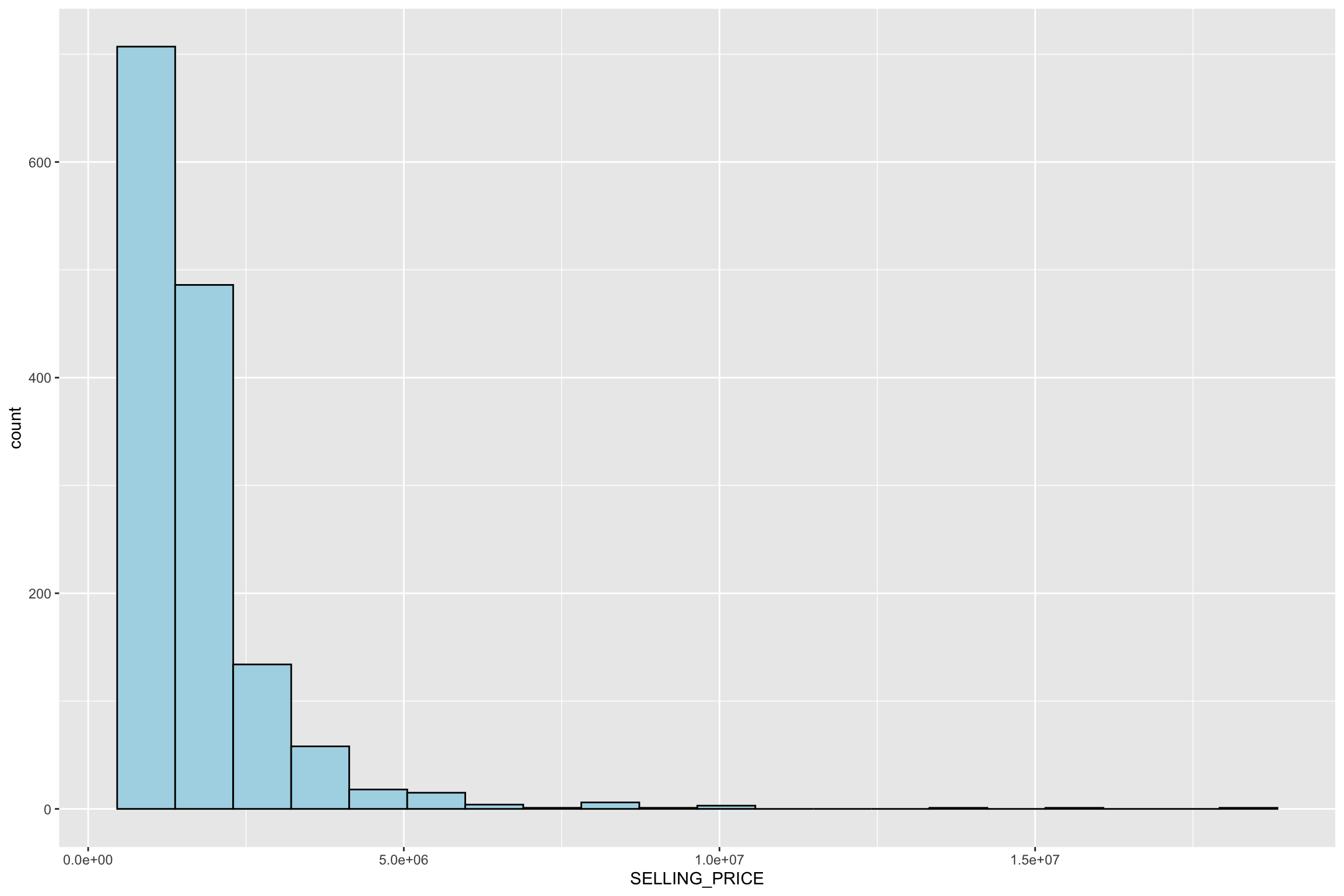
To plot the distribution of SELLING_PRICE by using histograms:
ggplot(data=condo_resale.sf, aes(x=`SELLING_PRICE`)) +
geom_histogram(bins=20, color="black", fill="light blue")
Note
Observations:
- A right skewed distribution.
- This means that more condominium units were transacted at relative lower prices.
- Statistically, the skewed distribution can be normalised by using log transformation.
condo_resale.sf <- condo_resale.sf %>%
mutate(`LOG_SELLING_PRICE` = log(SELLING_PRICE))
ggplot(data=condo_resale.sf, aes(x=`LOG_SELLING_PRICE`)) +
geom_histogram(bins=20, color="black", fill="light blue")
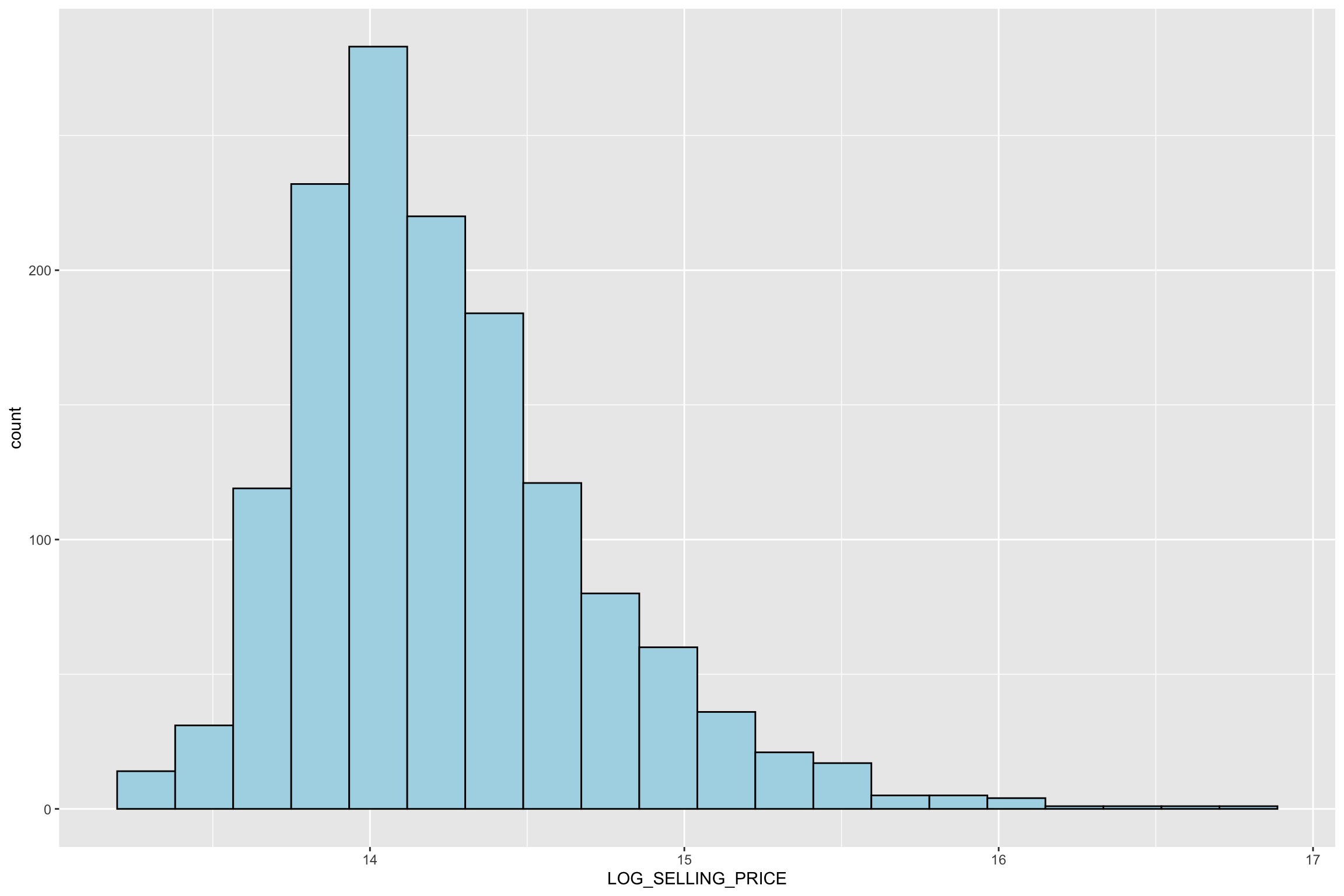
Notice that the distribution is relatively less skewed after the transformation.
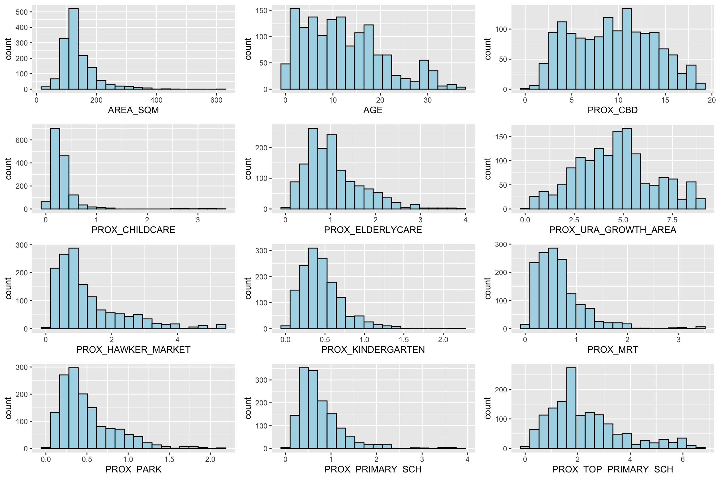
8.3 Multiple Histogram Plots for Variable Distribution
In this section, we will create multiple histograms (also known as
a trellis plot or small multiples) to visualize the distribution
of several variables. We will use the
ggarrange() function from the
ggpubr
package to organize these histograms into a 3-column by 4-row grid
layout.
Show the code
# List of variables to plot
variables <- c("AREA_SQM", "AGE", "PROX_CBD", "PROX_CHILDCARE",
"PROX_ELDERLYCARE", "PROX_URA_GROWTH_AREA",
"PROX_HAWKER_MARKET", "PROX_KINDERGARTEN",
"PROX_MRT", "PROX_PARK", "PROX_PRIMARY_SCH",
"PROX_TOP_PRIMARY_SCH")
histograms <- lapply(variables, function(var) {
ggplot(condo_resale.sf, aes_string(x = var)) +
geom_histogram(bins = 20, color = "black", fill = "lightblue")
})
ggarrange(plotlist = histograms, ncol = 3, nrow = 4)
8.4 Drawing a Statistical Point Map
In this section, we will visualize the geospatial distribution of condominium resale prices in Singapore.
-
The map will be prepared by using tmap package.
-
tmap_mode("view")to use the interactive mode of tmap
-
-
Then, create an interactive point symbol map
-
tm_dots()is used instead oftm_bubbles() -
set.zoom.limitsargument oftm_view()sets the minimum and maximum zoom level to 11 and 14 respectively.
-
-
Lastly,
tmap_mode("plot")to display plot mode
Show the code
tmap_mode("view")
tmap_options(check.and.fix = TRUE)
tm_shape(mpsz_svy21)+
tm_polygons() +
tm_shape(condo_resale.sf) +
tm_dots(col = "SELLING_PRICE",
alpha = 0.6,
style="quantile") +
tm_view(set.zoom.limits = c(11,14))Show the code
tmap_mode("plot")9 Hedonic Pricing Model in R
In this section, we will build a hedonic pricing model for
condominium resale units using the
lm()
function from base R.
9.1 Simple Linear Regression
We start by modeling SELLING_PRICE as the dependent variable and AREA_SQM as the independent variable.
Call:
lm(formula = SELLING_PRICE ~ AREA_SQM, data = condo_resale.sf)
Residuals:
Min 1Q Median 3Q Max
-3695815 -391764 -87517 258900 13503875
Coefficients:
Estimate Std. Error t value Pr(>|t|)
(Intercept) -258121.1 63517.2 -4.064 5.09e-05 ***
AREA_SQM 14719.0 428.1 34.381 < 2e-16 ***
---
Signif. codes: 0 '***' 0.001 '**' 0.01 '*' 0.05 '.' 0.1 ' ' 1
Residual standard error: 942700 on 1434 degrees of freedom
Multiple R-squared: 0.4518, Adjusted R-squared: 0.4515
F-statistic: 1182 on 1 and 1434 DF, p-value: < 2.2e-16Note
Observations:
-
The model equation is:
SELLING_PRICE = -258121.1 + 14719 * AREA_SQM - R-squared: 0.4518, indicating the model explains 45% of the variation in resale prices.
- P-value: The very small p-value (< 0.0001) indicates strong evidence to reject the null hypothesis, suggesting the model is a good fit.
- Coefficients: Both the intercept and slope have p-values < 0.001, confirming that the parameters are significant predictors.
To visualize the fit, we can plot the data and the regression line:
ggplot(data = condo_resale.sf, aes(x = AREA_SQM, y = SELLING_PRICE)) +
geom_point() +
geom_smooth(method = lm)
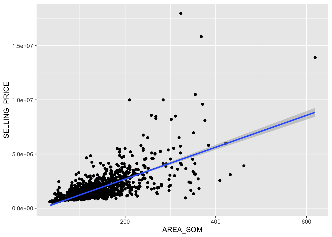
This scatterplot with a fitted regression line highlights some high-price outliers in the dataset.
9.2 Multiple Linear Regression
9.2.1 Checking for Multicollinearity
Before building a multiple regression model, it is essential to ensure that the independent variables are not highly correlated, as this can lead to multicollinearity, which compromises the model’s quality.
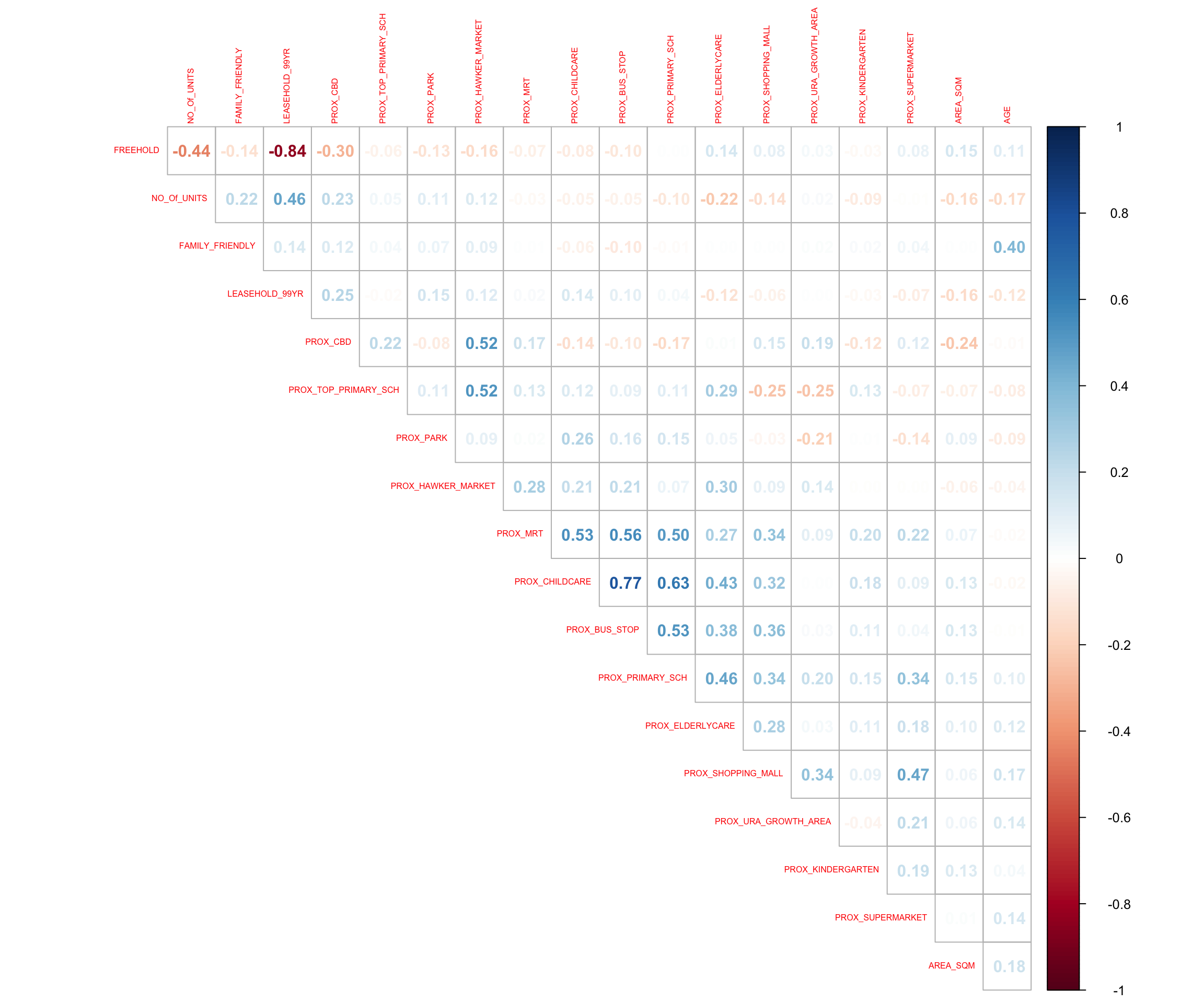
A correlation matrix is useful for visualizing relationships between variables. In this case, we use the corrplot package to plot a correlation matrix for the independent variables.
corrplot(cor(condo_resale[, 5:23]), diag = FALSE, order = "AOE",
tl.pos = "td", tl.cex = 0.5, method = "number", type = "upper")
Tip
Matrix reorder is very important for mining the hiden structure and patter in the matrix. There are four methods in corrplot (parameter order), named “AOE”, “FPC”, “hclust”, “alphabet”. In the code chunk above, AOE order is used. It orders the variables by using the angular order of the eigenvectors method suggested by Michael Friendly.
Note
Observations:
- From the matrix, we observe that Freehold and LEASE_99YEAR are highly correlated, so only Freehold will be included in the model.
9.3 Building the Multiple Linear Regression Model
We now build a hedonic pricing model using multiple linear regression. The model predicts SELLING_PRICE based on several property characteristics.
condo.mlr <- lm(SELLING_PRICE ~ AREA_SQM + AGE +
PROX_CBD + PROX_CHILDCARE + PROX_ELDERLYCARE +
PROX_URA_GROWTH_AREA + PROX_HAWKER_MARKET +
PROX_KINDERGARTEN + PROX_MRT + PROX_PARK +
PROX_PRIMARY_SCH + PROX_TOP_PRIMARY_SCH +
PROX_SHOPPING_MALL + PROX_SUPERMARKET +
PROX_BUS_STOP + NO_Of_UNITS + FAMILY_FRIENDLY + FREEHOLD,
data = condo_resale.sf)
summary(condo.mlr)
Call:
lm(formula = SELLING_PRICE ~ AREA_SQM + AGE + PROX_CBD + PROX_CHILDCARE +
PROX_ELDERLYCARE + PROX_URA_GROWTH_AREA + PROX_HAWKER_MARKET +
PROX_KINDERGARTEN + PROX_MRT + PROX_PARK + PROX_PRIMARY_SCH +
PROX_TOP_PRIMARY_SCH + PROX_SHOPPING_MALL + PROX_SUPERMARKET +
PROX_BUS_STOP + NO_Of_UNITS + FAMILY_FRIENDLY + FREEHOLD,
data = condo_resale.sf)
Residuals:
Min 1Q Median 3Q Max
-3475964 -293923 -23069 241043 12260381
Coefficients:
Estimate Std. Error t value Pr(>|t|)
(Intercept) 481728.40 121441.01 3.967 7.65e-05 ***
AREA_SQM 12708.32 369.59 34.385 < 2e-16 ***
AGE -24440.82 2763.16 -8.845 < 2e-16 ***
PROX_CBD -78669.78 6768.97 -11.622 < 2e-16 ***
PROX_CHILDCARE -351617.91 109467.25 -3.212 0.00135 **
PROX_ELDERLYCARE 171029.42 42110.51 4.061 5.14e-05 ***
PROX_URA_GROWTH_AREA 38474.53 12523.57 3.072 0.00217 **
PROX_HAWKER_MARKET 23746.10 29299.76 0.810 0.41782
PROX_KINDERGARTEN 147468.99 82668.87 1.784 0.07466 .
PROX_MRT -314599.68 57947.44 -5.429 6.66e-08 ***
PROX_PARK 563280.50 66551.68 8.464 < 2e-16 ***
PROX_PRIMARY_SCH 180186.08 65237.95 2.762 0.00582 **
PROX_TOP_PRIMARY_SCH 2280.04 20410.43 0.112 0.91107
PROX_SHOPPING_MALL -206604.06 42840.60 -4.823 1.57e-06 ***
PROX_SUPERMARKET -44991.80 77082.64 -0.584 0.55953
PROX_BUS_STOP 683121.35 138353.28 4.938 8.85e-07 ***
NO_Of_UNITS -231.18 89.03 -2.597 0.00951 **
FAMILY_FRIENDLY 140340.77 47020.55 2.985 0.00289 **
FREEHOLD 359913.01 49220.22 7.312 4.38e-13 ***
---
Signif. codes: 0 '***' 0.001 '**' 0.01 '*' 0.05 '.' 0.1 ' ' 1
Residual standard error: 755800 on 1417 degrees of freedom
Multiple R-squared: 0.6518, Adjusted R-squared: 0.6474
F-statistic: 147.4 on 18 and 1417 DF, p-value: < 2.2e-16Note
Observations:
-
Significant predictors:
- AREA_SQM (positive): Larger units have higher selling prices.
- AGE (negative): Older units tend to sell for less.
- PROX_CBD (negative): Proximity to the central business district reduces selling prices.
- PROX_PARK (positive): Proximity to parks increases resale prices.
- FREEHOLD (positive): Freehold properties sell for more than leasehold properties.
-
Non-significant predictors (p > 0.05):
- PROX_HAWKER_MARKET, PROX_TOP_PRIMARY_SCH, PROX_SUPERMARKET show weak or no significant relationship with SELLING_PRICE.
9.4 Revising the Hedonic Pricing Model
After reviewing the initial model, we will now remove non-significant variables to improve the model. The revised multiple linear regression model is calibrated as follows:
condo.mlr1 <- lm(formula = SELLING_PRICE ~ AREA_SQM + AGE +
PROX_CBD + PROX_CHILDCARE + PROX_ELDERLYCARE +
PROX_URA_GROWTH_AREA + PROX_MRT + PROX_PARK +
PROX_PRIMARY_SCH + PROX_SHOPPING_MALL + PROX_BUS_STOP +
NO_Of_UNITS + FAMILY_FRIENDLY + FREEHOLD,
data = condo_resale.sf)
ols_regress(condo.mlr1) Model Summary
-----------------------------------------------------------------------------
R 0.807 RMSE 751998.679
R-Squared 0.651 MSE 571471422208.592
Adj. R-Squared 0.647 Coef. Var 43.168
Pred R-Squared 0.638 AIC 42966.758
MAE 414819.628 SBC 43051.072
-----------------------------------------------------------------------------
RMSE: Root Mean Square Error
MSE: Mean Square Error
MAE: Mean Absolute Error
AIC: Akaike Information Criteria
SBC: Schwarz Bayesian Criteria
ANOVA
--------------------------------------------------------------------------------
Sum of
Squares DF Mean Square F Sig.
--------------------------------------------------------------------------------
Regression 1.512586e+15 14 1.080418e+14 189.059 0.0000
Residual 8.120609e+14 1421 571471422208.592
Total 2.324647e+15 1435
--------------------------------------------------------------------------------
Parameter Estimates
-----------------------------------------------------------------------------------------------------------------
model Beta Std. Error Std. Beta t Sig lower upper
-----------------------------------------------------------------------------------------------------------------
(Intercept) 527633.222 108183.223 4.877 0.000 315417.244 739849.200
AREA_SQM 12777.523 367.479 0.584 34.771 0.000 12056.663 13498.382
AGE -24687.739 2754.845 -0.167 -8.962 0.000 -30091.739 -19283.740
PROX_CBD -77131.323 5763.125 -0.263 -13.384 0.000 -88436.469 -65826.176
PROX_CHILDCARE -318472.751 107959.512 -0.084 -2.950 0.003 -530249.889 -106695.613
PROX_ELDERLYCARE 185575.623 39901.864 0.090 4.651 0.000 107302.737 263848.510
PROX_URA_GROWTH_AREA 39163.254 11754.829 0.060 3.332 0.001 16104.571 62221.936
PROX_MRT -294745.107 56916.367 -0.112 -5.179 0.000 -406394.234 -183095.980
PROX_PARK 570504.807 65507.029 0.150 8.709 0.000 442003.938 699005.677
PROX_PRIMARY_SCH 159856.136 60234.599 0.062 2.654 0.008 41697.849 278014.424
PROX_SHOPPING_MALL -220947.251 36561.832 -0.115 -6.043 0.000 -292668.213 -149226.288
PROX_BUS_STOP 682482.221 134513.243 0.134 5.074 0.000 418616.359 946348.082
NO_Of_UNITS -245.480 87.947 -0.053 -2.791 0.005 -418.000 -72.961
FAMILY_FRIENDLY 146307.576 46893.021 0.057 3.120 0.002 54320.593 238294.560
FREEHOLD 350599.812 48506.485 0.136 7.228 0.000 255447.802 445751.821
-----------------------------------------------------------------------------------------------------------------
9.5 Publication-Ready
Table with gtsummary
The gtsummary package provides an elegant way to create publication-ready regression tables. The following code generates a formatted regression report:
tbl_regression(condo.mlr1, intercept = TRUE)|
Characteristic |
Beta |
95% CI 1 |
p-value |
|---|---|---|---|
| (Intercept) | 527,633 | 315,417, 739,849 | <0.001 |
| AREA_SQM | 12,778 | 12,057, 13,498 | <0.001 |
| AGE | -24,688 | -30,092, -19,284 | <0.001 |
| PROX_CBD | -77,131 | -88,436, -65,826 | <0.001 |
| PROX_CHILDCARE | -318,473 | -530,250, -106,696 | 0.003 |
| PROX_ELDERLYCARE | 185,576 | 107,303, 263,849 | <0.001 |
| PROX_URA_GROWTH_AREA | 39,163 | 16,105, 62,222 | <0.001 |
| PROX_MRT | -294,745 | -406,394, -183,096 | <0.001 |
| PROX_PARK | 570,505 | 442,004, 699,006 | <0.001 |
| PROX_PRIMARY_SCH | 159,856 | 41,698, 278,014 | 0.008 |
| PROX_SHOPPING_MALL | -220,947 | -292,668, -149,226 | <0.001 |
| PROX_BUS_STOP | 682,482 | 418,616, 946,348 | <0.001 |
| NO_Of_UNITS | -245 | -418, -73 | 0.005 |
| FAMILY_FRIENDLY | 146,308 | 54,321, 238,295 | 0.002 |
| FREEHOLD | 350,600 | 255,448, 445,752 | <0.001 |
|
1
CI = Confidence Interval |
|||
You can further enhance the report by adding model statistics
using add_glance_table() or
add_glance_source_note():
9.5.1 Checking for Multicollinearity
We can check for multicollinearity using the
olsrr package’s
ols_vif_tol() function:
ols_vif_tol(condo.mlr1) Variables Tolerance VIF
1 AREA_SQM 0.8728554 1.145665
2 AGE 0.7071275 1.414172
3 PROX_CBD 0.6356147 1.573280
4 PROX_CHILDCARE 0.3066019 3.261559
5 PROX_ELDERLYCARE 0.6598479 1.515501
6 PROX_URA_GROWTH_AREA 0.7510311 1.331503
7 PROX_MRT 0.5236090 1.909822
8 PROX_PARK 0.8279261 1.207837
9 PROX_PRIMARY_SCH 0.4524628 2.210126
10 PROX_SHOPPING_MALL 0.6738795 1.483945
11 PROX_BUS_STOP 0.3514118 2.845664
12 NO_Of_UNITS 0.6901036 1.449058
13 FAMILY_FRIENDLY 0.7244157 1.380423
14 FREEHOLD 0.6931163 1.442759Note
Observations:
Since the VIF values are all below 10, there is no indication of multicollinearity among the independent variables.
9.5.2 Test for Non-Linearity
In multiple linear regression, it is important for us to test the assumption that linearity and additivity of the relationship between dependent and independent variables.
To test the linearity assumption, we use the
ols_plot_resid_fit() function.
ols_plot_resid_fit(condo.mlr1)
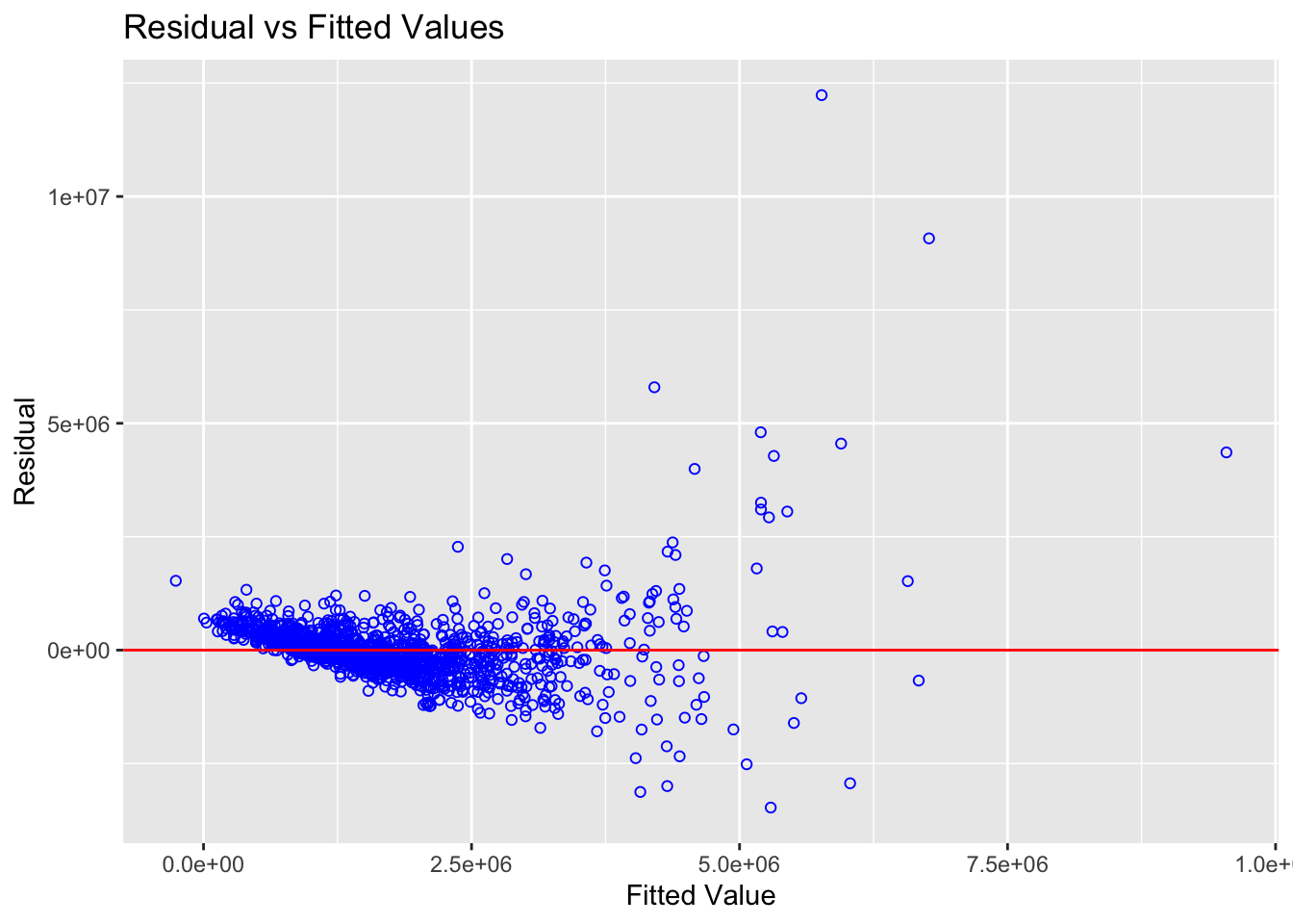
Note
Observations:
Most points are scattered around the 0 line, hence we can safely conclude that the relationships between the dependent variable and independent variables are linear.
9.5.3 Test for Normality Assumption
We can assess the normality of residuals with a histogram:
ols_plot_resid_hist(condo.mlr1)
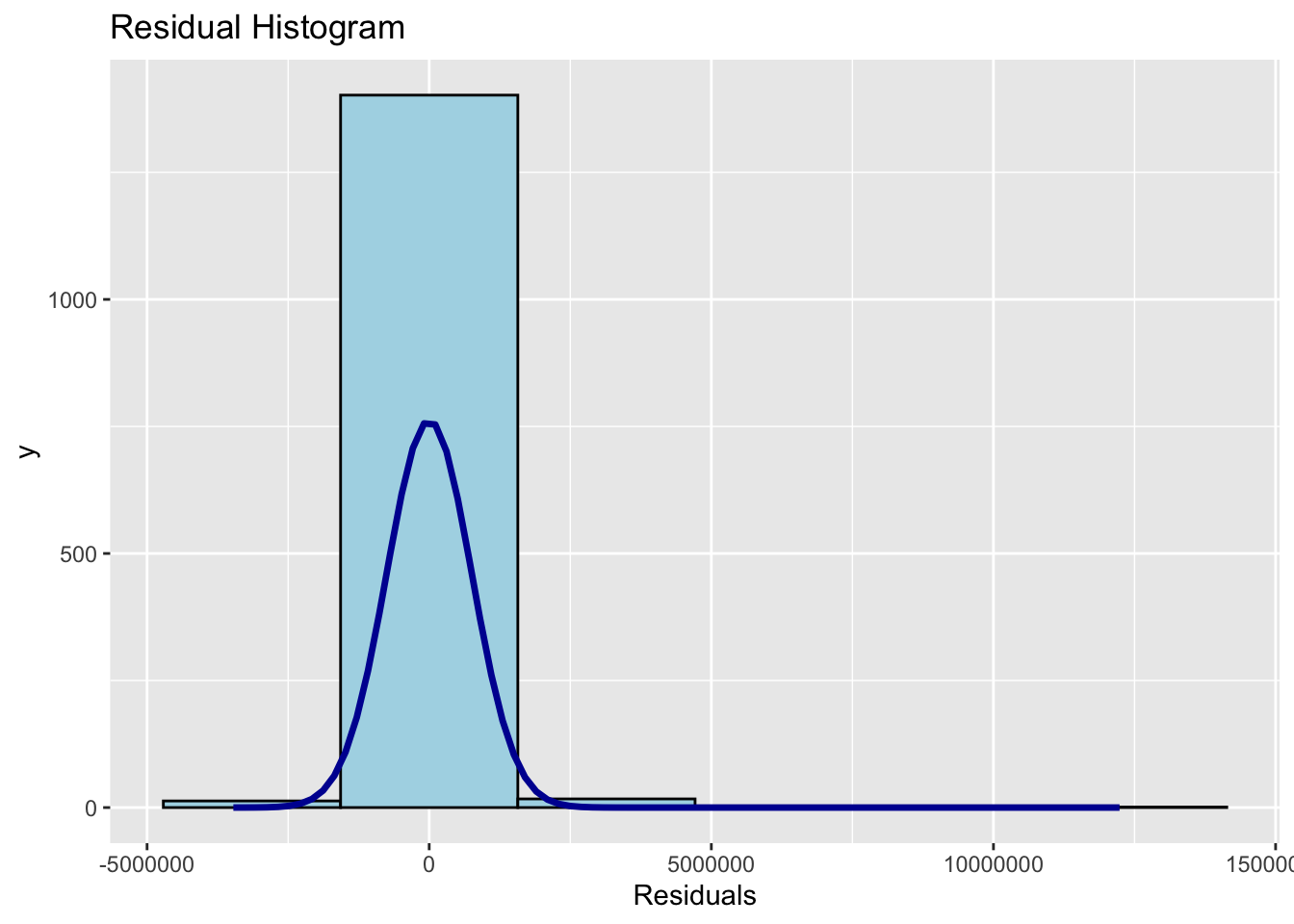
The residuals appear normally distributed. For a formal test, we
can use ols_test_normality():
ols_test_normality(condo.mlr1)-----------------------------------------------
Test Statistic pvalue
-----------------------------------------------
Shapiro-Wilk 0.6856 0.0000
Kolmogorov-Smirnov 0.1366 0.0000
Cramer-von Mises 121.0768 0.0000
Anderson-Darling 67.9551 0.0000
-----------------------------------------------Note
Observations:
The summary table above reveals that the p-values of the four tests are way smaller than the alpha value of 0.05. Hence we will reject the null hypothesis and infer that there is statistical evidence that the residual are not normally distributed.
9.5.4 Testing for Spatial Autocorrelation
Since the hedonic model involves geographically referenced data, it is important to visualize the residuals and test for spatial autocorrelation.
First, we export the residuals from the hedonic pricing model into a data frame.
mlr.output <- as.data.frame(condo.mlr1$residuals)Next, we join the residuals with the condo_resale.sf spatial data frame:
condo_resale.res.sf <- cbind(condo_resale.sf, condo.mlr1$residuals) %>%
rename(MLR_RES = condo.mlr1.residuals)We convert the condo_resale.res.sf from an sf object to a SpatialPointsDataFrame for use with the spdep package:
condo_resale.sp <- as_Spatial(condo_resale.res.sf)
condo_resale.spclass : SpatialPointsDataFrame
features : 1436
extent : 14940.85, 43352.45, 24765.67, 48382.81 (xmin, xmax, ymin, ymax)
crs : +proj=tmerc +lat_0=1.36666666666667 +lon_0=103.833333333333 +k=1 +x_0=28001.642 +y_0=38744.572 +ellps=WGS84 +towgs84=0,0,0,0,0,0,0 +units=m +no_defs
variables : 23
names : POSTCODE, SELLING_PRICE, AREA_SQM, AGE, PROX_CBD, PROX_CHILDCARE, PROX_ELDERLYCARE, PROX_URA_GROWTH_AREA, PROX_HAWKER_MARKET, PROX_KINDERGARTEN, PROX_MRT, PROX_PARK, PROX_PRIMARY_SCH, PROX_TOP_PRIMARY_SCH, PROX_SHOPPING_MALL, ...
min values : 18965, 540000, 34, 0, 0.386916393, 0.004927023, 0.054508623, 0.214539508, 0.051817113, 0.004927023, 0.052779424, 0.029064164, 0.077106132, 0.077106132, 0, ...
max values : 828833, 1.8e+07, 619, 37, 19.18042832, 3.46572633, 3.949157205, 9.15540001, 5.374348075, 2.229045366, 3.48037319, 2.16104919, 3.928989144, 6.748192062, 3.477433767, ... Using tmap, we visualize the spatial distribution of the residuals:
tmap_mode("view")
tm_shape(mpsz_svy21) +
tmap_options(check.and.fix = TRUE) +
tm_polygons(alpha = 0.4) +
tm_shape(condo_resale.res.sf) +
tm_dots(col = "MLR_RES", alpha = 0.6, style = "quantile") +
tm_view(set.zoom.limits = c(11, 14))tmap_mode("plot")Note
Observations:
The figure above reveal that there is sign of spatial autocorrelation.
To formally test for spatial autocorrelation using Moran’s I Test, we first compute a distance-based weight matrix:
nb <- dnearneigh(coordinates(condo_resale.sp), 0, 1500, longlat = FALSE)
summary(nb)Neighbour list object:
Number of regions: 1436
Number of nonzero links: 66266
Percentage nonzero weights: 3.213526
Average number of links: 46.14624
10 disjoint connected subgraphs
Link number distribution:
1 3 5 7 9 10 11 12 13 14 15 16 17 18 19 20 21 22 23 24
3 3 9 4 3 15 10 19 17 45 19 5 14 29 19 6 35 45 18 47
25 26 27 28 29 30 31 32 33 34 35 36 37 38 39 40 41 42 43 44
16 43 22 26 21 11 9 23 22 13 16 25 21 37 16 18 8 21 4 12
45 46 47 48 49 50 51 52 53 54 55 56 57 58 59 60 61 62 63 64
8 36 18 14 14 43 11 12 8 13 12 13 4 5 6 12 11 20 29 33
65 66 67 68 69 70 71 72 73 74 75 76 77 78 79 80 81 82 83 84
15 20 10 14 15 15 11 16 12 10 8 19 12 14 9 8 4 13 11 6
85 86 87 88 89 90 91 92 93 94 95 96 97 98 99 100 101 102 103 104
4 9 4 4 4 6 2 16 9 4 5 9 3 9 4 2 1 2 1 1
105 106 107 108 109 110 112 116 125
1 5 9 2 1 3 1 1 1
3 least connected regions:
193 194 277 with 1 link
1 most connected region:
285 with 125 linksConvert the neighbor list into spatial weights:
nb_lw <- nb2listw(nb, style = 'W')
summary(nb_lw)Characteristics of weights list object:
Neighbour list object:
Number of regions: 1436
Number of nonzero links: 66266
Percentage nonzero weights: 3.213526
Average number of links: 46.14624
10 disjoint connected subgraphs
Link number distribution:
1 3 5 7 9 10 11 12 13 14 15 16 17 18 19 20 21 22 23 24
3 3 9 4 3 15 10 19 17 45 19 5 14 29 19 6 35 45 18 47
25 26 27 28 29 30 31 32 33 34 35 36 37 38 39 40 41 42 43 44
16 43 22 26 21 11 9 23 22 13 16 25 21 37 16 18 8 21 4 12
45 46 47 48 49 50 51 52 53 54 55 56 57 58 59 60 61 62 63 64
8 36 18 14 14 43 11 12 8 13 12 13 4 5 6 12 11 20 29 33
65 66 67 68 69 70 71 72 73 74 75 76 77 78 79 80 81 82 83 84
15 20 10 14 15 15 11 16 12 10 8 19 12 14 9 8 4 13 11 6
85 86 87 88 89 90 91 92 93 94 95 96 97 98 99 100 101 102 103 104
4 9 4 4 4 6 2 16 9 4 5 9 3 9 4 2 1 2 1 1
105 106 107 108 109 110 112 116 125
1 5 9 2 1 3 1 1 1
3 least connected regions:
193 194 277 with 1 link
1 most connected region:
285 with 125 links
Weights style: W
Weights constants summary:
n nn S0 S1 S2
W 1436 2062096 1436 94.81916 5798.341Finally, perform Moran’s I test on the model residuals:
lm.morantest(condo.mlr1, nb_lw)
Global Moran I for regression residuals
data:
model: lm(formula = SELLING_PRICE ~ AREA_SQM + AGE + PROX_CBD +
PROX_CHILDCARE + PROX_ELDERLYCARE + PROX_URA_GROWTH_AREA + PROX_MRT +
PROX_PARK + PROX_PRIMARY_SCH + PROX_SHOPPING_MALL + PROX_BUS_STOP +
NO_Of_UNITS + FAMILY_FRIENDLY + FREEHOLD, data = condo_resale.sf)
weights: nb_lw
Moran I statistic standard deviate = 24.366, p-value < 2.2e-16
alternative hypothesis: greater
sample estimates:
Observed Moran I Expectation Variance
1.438876e-01 -5.487594e-03 3.758259e-05 Note
Observations:
- P-value: The p-value is extremely small (< 0.05), leading us to reject the null hypothesis that residuals are randomly distributed.
- Observed Moran’s I: The value of 0.1424418 (greater than 0) indicates that residuals show a clustered pattern, confirming the presence of spatial autocorrelation.
10 Building Hedonic Pricing Models using GWmodel
In this section, we will model hedonic pricing using both fixed and adaptive bandwidth schemes.
10.1 Building Fixed Bandwidth GWR Model
10.1.1 Computing Fixed Bandwidth
We use the bw.gwr() function from the
GWModel package to determine the optimal fixed
bandwidth for the model.
Setting adaptive = FALSE ensures that we are
calculating a fixed bandwidth. There are two possible approaches
for determining the stopping rule:
CV cross-validation and AICc.
In this case, we use the cross-validation approach (approach = "CV").
bw.fixed <- bw.gwr(formula = SELLING_PRICE ~ AREA_SQM + AGE + PROX_CBD +
PROX_CHILDCARE + PROX_ELDERLYCARE + PROX_URA_GROWTH_AREA +
PROX_MRT + PROX_PARK + PROX_PRIMARY_SCH +
PROX_SHOPPING_MALL + PROX_BUS_STOP + NO_Of_UNITS +
FAMILY_FRIENDLY + FREEHOLD,
data = condo_resale.sp,
approach = "CV",
kernel = "gaussian",
adaptive = FALSE,
longlat = FALSE)Fixed bandwidth: 17660.96 CV score: 8.259118e+14
Fixed bandwidth: 10917.26 CV score: 7.970454e+14
Fixed bandwidth: 6749.419 CV score: 7.273273e+14
Fixed bandwidth: 4173.553 CV score: 6.300006e+14
Fixed bandwidth: 2581.58 CV score: 5.404958e+14
Fixed bandwidth: 1597.687 CV score: 4.857515e+14
Fixed bandwidth: 989.6077 CV score: 4.722431e+14
Fixed bandwidth: 613.7939 CV score: 1.379526e+16
Fixed bandwidth: 1221.873 CV score: 4.778717e+14
Fixed bandwidth: 846.0596 CV score: 4.791629e+14
Fixed bandwidth: 1078.325 CV score: 4.751406e+14
Fixed bandwidth: 934.7772 CV score: 4.72518e+14
Fixed bandwidth: 1023.495 CV score: 4.730305e+14
Fixed bandwidth: 968.6643 CV score: 4.721317e+14
Fixed bandwidth: 955.7206 CV score: 4.722072e+14
Fixed bandwidth: 976.6639 CV score: 4.721387e+14
Fixed bandwidth: 963.7202 CV score: 4.721484e+14
Fixed bandwidth: 971.7199 CV score: 4.721293e+14
Fixed bandwidth: 973.6083 CV score: 4.721309e+14
Fixed bandwidth: 970.5527 CV score: 4.721295e+14
Fixed bandwidth: 972.4412 CV score: 4.721296e+14
Fixed bandwidth: 971.2741 CV score: 4.721292e+14
Fixed bandwidth: 970.9985 CV score: 4.721293e+14
Fixed bandwidth: 971.4443 CV score: 4.721292e+14
Fixed bandwidth: 971.5496 CV score: 4.721293e+14
Fixed bandwidth: 971.3793 CV score: 4.721292e+14
Fixed bandwidth: 971.3391 CV score: 4.721292e+14
Fixed bandwidth: 971.3143 CV score: 4.721292e+14
Fixed bandwidth: 971.3545 CV score: 4.721292e+14
Fixed bandwidth: 971.3296 CV score: 4.721292e+14
Fixed bandwidth: 971.345 CV score: 4.721292e+14
Fixed bandwidth: 971.3355 CV score: 4.721292e+14
Fixed bandwidth: 971.3413 CV score: 4.721292e+14
Fixed bandwidth: 971.3377 CV score: 4.721292e+14
Fixed bandwidth: 971.34 CV score: 4.721292e+14
Fixed bandwidth: 971.3405 CV score: 4.721292e+14
Fixed bandwidth: 971.3396 CV score: 4.721292e+14
Fixed bandwidth: 971.3402 CV score: 4.721292e+14
Fixed bandwidth: 971.3398 CV score: 4.721292e+14
Fixed bandwidth: 971.34 CV score: 4.721292e+14
Fixed bandwidth: 971.3399 CV score: 4.721292e+14
Fixed bandwidth: 971.34 CV score: 4.721292e+14 The recommended bandwidth is 971.34 meters.
Note
Quiz Answer:
The bandwidth is in meters because the model is using
projected coordinates, SVY21, where distances are measured
in meters.
10.1.2 GWModel Method - Fixed Bandwidth
We can now calibrate the GWR model using a fixed bandwidth and a Gaussian kernel with the following code:
gwr.fixed <- gwr.basic(formula = SELLING_PRICE ~ AREA_SQM + AGE + PROX_CBD +
PROX_CHILDCARE + PROX_ELDERLYCARE + PROX_URA_GROWTH_AREA +
PROX_MRT + PROX_PARK + PROX_PRIMARY_SCH +
PROX_SHOPPING_MALL + PROX_BUS_STOP + NO_Of_UNITS +
FAMILY_FRIENDLY + FREEHOLD,
data = condo_resale.sp,
bw = bw.fixed,
kernel = 'gaussian',
longlat = FALSE)
gwr.fixed ***********************************************************************
* Package GWmodel *
***********************************************************************
Program starts at: 2024-10-14 19:55:45.822271
Call:
gwr.basic(formula = SELLING_PRICE ~ AREA_SQM + AGE + PROX_CBD +
PROX_CHILDCARE + PROX_ELDERLYCARE + PROX_URA_GROWTH_AREA +
PROX_MRT + PROX_PARK + PROX_PRIMARY_SCH + PROX_SHOPPING_MALL +
PROX_BUS_STOP + NO_Of_UNITS + FAMILY_FRIENDLY + FREEHOLD,
data = condo_resale.sp, bw = bw.fixed, kernel = "gaussian",
longlat = FALSE)
Dependent (y) variable: SELLING_PRICE
Independent variables: AREA_SQM AGE PROX_CBD PROX_CHILDCARE PROX_ELDERLYCARE PROX_URA_GROWTH_AREA PROX_MRT PROX_PARK PROX_PRIMARY_SCH PROX_SHOPPING_MALL PROX_BUS_STOP NO_Of_UNITS FAMILY_FRIENDLY FREEHOLD
Number of data points: 1436
***********************************************************************
* Results of Global Regression *
***********************************************************************
Call:
lm(formula = formula, data = data)
Residuals:
Min 1Q Median 3Q Max
-3470778 -298119 -23481 248917 12234210
Coefficients:
Estimate Std. Error t value Pr(>|t|)
(Intercept) 527633.22 108183.22 4.877 1.20e-06 ***
AREA_SQM 12777.52 367.48 34.771 < 2e-16 ***
AGE -24687.74 2754.84 -8.962 < 2e-16 ***
PROX_CBD -77131.32 5763.12 -13.384 < 2e-16 ***
PROX_CHILDCARE -318472.75 107959.51 -2.950 0.003231 **
PROX_ELDERLYCARE 185575.62 39901.86 4.651 3.61e-06 ***
PROX_URA_GROWTH_AREA 39163.25 11754.83 3.332 0.000885 ***
PROX_MRT -294745.11 56916.37 -5.179 2.56e-07 ***
PROX_PARK 570504.81 65507.03 8.709 < 2e-16 ***
PROX_PRIMARY_SCH 159856.14 60234.60 2.654 0.008046 **
PROX_SHOPPING_MALL -220947.25 36561.83 -6.043 1.93e-09 ***
PROX_BUS_STOP 682482.22 134513.24 5.074 4.42e-07 ***
NO_Of_UNITS -245.48 87.95 -2.791 0.005321 **
FAMILY_FRIENDLY 146307.58 46893.02 3.120 0.001845 **
FREEHOLD 350599.81 48506.48 7.228 7.98e-13 ***
---Significance stars
Signif. codes: 0 '***' 0.001 '**' 0.01 '*' 0.05 '.' 0.1 ' ' 1
Residual standard error: 756000 on 1421 degrees of freedom
Multiple R-squared: 0.6507
Adjusted R-squared: 0.6472
F-statistic: 189.1 on 14 and 1421 DF, p-value: < 2.2e-16
***Extra Diagnostic information
Residual sum of squares: 8.120609e+14
Sigma(hat): 752522.9
AIC: 42966.76
AICc: 42967.14
BIC: 41731.39
***********************************************************************
* Results of Geographically Weighted Regression *
***********************************************************************
*********************Model calibration information*********************
Kernel function: gaussian
Fixed bandwidth: 971.34
Regression points: the same locations as observations are used.
Distance metric: Euclidean distance metric is used.
****************Summary of GWR coefficient estimates:******************
Min. 1st Qu. Median 3rd Qu.
Intercept -3.5988e+07 -5.1998e+05 7.6780e+05 1.7412e+06
AREA_SQM 1.0003e+03 5.2758e+03 7.4740e+03 1.2301e+04
AGE -1.3475e+05 -2.0813e+04 -8.6260e+03 -3.7784e+03
PROX_CBD -7.7047e+07 -2.3608e+05 -8.3599e+04 3.4646e+04
PROX_CHILDCARE -6.0097e+06 -3.3667e+05 -9.7426e+04 2.9007e+05
PROX_ELDERLYCARE -3.5001e+06 -1.5970e+05 3.1970e+04 1.9577e+05
PROX_URA_GROWTH_AREA -3.0170e+06 -8.2013e+04 7.0749e+04 2.2612e+05
PROX_MRT -3.5282e+06 -6.5836e+05 -1.8833e+05 3.6922e+04
PROX_PARK -1.2062e+06 -2.1732e+05 3.5383e+04 4.1335e+05
PROX_PRIMARY_SCH -2.2695e+07 -1.7066e+05 4.8472e+04 5.1555e+05
PROX_SHOPPING_MALL -7.2585e+06 -1.6684e+05 -1.0517e+04 1.5923e+05
PROX_BUS_STOP -1.4676e+06 -4.5207e+04 3.7601e+05 1.1664e+06
NO_Of_UNITS -1.3170e+03 -2.4822e+02 -3.0846e+01 2.5496e+02
FAMILY_FRIENDLY -2.2749e+06 -1.1140e+05 7.6214e+03 1.6107e+05
FREEHOLD -9.2067e+06 3.8074e+04 1.5169e+05 3.7528e+05
Max.
Intercept 112794435
AREA_SQM 21575
AGE 434203
PROX_CBD 2704604
PROX_CHILDCARE 1654086
PROX_ELDERLYCARE 38867861
PROX_URA_GROWTH_AREA 78515805
PROX_MRT 3124325
PROX_PARK 18122439
PROX_PRIMARY_SCH 4637517
PROX_SHOPPING_MALL 1529953
PROX_BUS_STOP 11342209
NO_Of_UNITS 12907
FAMILY_FRIENDLY 1720745
FREEHOLD 6073642
************************Diagnostic information*************************
Number of data points: 1436
Effective number of parameters (2trace(S) - trace(S'S)): 438.3807
Effective degrees of freedom (n-2trace(S) + trace(S'S)): 997.6193
AICc (GWR book, Fotheringham, et al. 2002, p. 61, eq 2.33): 42263.61
AIC (GWR book, Fotheringham, et al. 2002,GWR p. 96, eq. 4.22): 41632.36
BIC (GWR book, Fotheringham, et al. 2002,GWR p. 61, eq. 2.34): 42515.71
Residual sum of squares: 2.534069e+14
R-square value: 0.8909912
Adjusted R-square value: 0.8430418
***********************************************************************
Program stops at: 2024-10-14 19:55:47.015626 Note
Observations:
The AICc for this fixed bandwidth GWR model is 42263.61, which is lower than the global multiple linear regression model (AICc = 42967.1), indicating a better fit.
10.2 Building Adaptive Bandwidth GWR Model
10.2.1 Computing the Adaptive Bandwidth
To compute the adaptive bandwidth, we set
adaptive = TRUE in the
bw.gwr() function:
bw.adaptive <- bw.gwr(formula = SELLING_PRICE ~ AREA_SQM + AGE +
PROX_CBD + PROX_CHILDCARE + PROX_ELDERLYCARE +
PROX_URA_GROWTH_AREA + PROX_MRT + PROX_PARK +
PROX_PRIMARY_SCH + PROX_SHOPPING_MALL + PROX_BUS_STOP +
NO_Of_UNITS + FAMILY_FRIENDLY + FREEHOLD,
data = condo_resale.sp,
approach = "CV",
kernel = "gaussian",
adaptive = TRUE,
longlat = FALSE)Adaptive bandwidth: 895 CV score: 7.952401e+14
Adaptive bandwidth: 561 CV score: 7.667364e+14
Adaptive bandwidth: 354 CV score: 6.953454e+14
Adaptive bandwidth: 226 CV score: 6.15223e+14
Adaptive bandwidth: 147 CV score: 5.674373e+14
Adaptive bandwidth: 98 CV score: 5.426745e+14
Adaptive bandwidth: 68 CV score: 5.168117e+14
Adaptive bandwidth: 49 CV score: 4.859631e+14
Adaptive bandwidth: 37 CV score: 4.646518e+14
Adaptive bandwidth: 30 CV score: 4.422088e+14
Adaptive bandwidth: 25 CV score: 4.430816e+14
Adaptive bandwidth: 32 CV score: 4.505602e+14
Adaptive bandwidth: 27 CV score: 4.462172e+14
Adaptive bandwidth: 30 CV score: 4.422088e+14 Note
Observations:
The result suggests using 30 data points for the adaptive bandwidth.
10.2.2 Constructing the Adaptive Bandwidth GWR Model
We can now calibrate the GWR model with the adaptive bandwidth:
gwr.adaptive <- gwr.basic(formula = SELLING_PRICE ~ AREA_SQM + AGE +
PROX_CBD + PROX_CHILDCARE + PROX_ELDERLYCARE +
PROX_URA_GROWTH_AREA + PROX_MRT + PROX_PARK +
PROX_PRIMARY_SCH + PROX_SHOPPING_MALL + PROX_BUS_STOP +
NO_Of_UNITS + FAMILY_FRIENDLY + FREEHOLD,
data = condo_resale.sp,
bw = bw.adaptive,
kernel = 'gaussian',
adaptive = TRUE,
longlat = FALSE)
gwr.adaptive ***********************************************************************
* Package GWmodel *
***********************************************************************
Program starts at: 2024-10-14 19:55:56.103874
Call:
gwr.basic(formula = SELLING_PRICE ~ AREA_SQM + AGE + PROX_CBD +
PROX_CHILDCARE + PROX_ELDERLYCARE + PROX_URA_GROWTH_AREA +
PROX_MRT + PROX_PARK + PROX_PRIMARY_SCH + PROX_SHOPPING_MALL +
PROX_BUS_STOP + NO_Of_UNITS + FAMILY_FRIENDLY + FREEHOLD,
data = condo_resale.sp, bw = bw.adaptive, kernel = "gaussian",
adaptive = TRUE, longlat = FALSE)
Dependent (y) variable: SELLING_PRICE
Independent variables: AREA_SQM AGE PROX_CBD PROX_CHILDCARE PROX_ELDERLYCARE PROX_URA_GROWTH_AREA PROX_MRT PROX_PARK PROX_PRIMARY_SCH PROX_SHOPPING_MALL PROX_BUS_STOP NO_Of_UNITS FAMILY_FRIENDLY FREEHOLD
Number of data points: 1436
***********************************************************************
* Results of Global Regression *
***********************************************************************
Call:
lm(formula = formula, data = data)
Residuals:
Min 1Q Median 3Q Max
-3470778 -298119 -23481 248917 12234210
Coefficients:
Estimate Std. Error t value Pr(>|t|)
(Intercept) 527633.22 108183.22 4.877 1.20e-06 ***
AREA_SQM 12777.52 367.48 34.771 < 2e-16 ***
AGE -24687.74 2754.84 -8.962 < 2e-16 ***
PROX_CBD -77131.32 5763.12 -13.384 < 2e-16 ***
PROX_CHILDCARE -318472.75 107959.51 -2.950 0.003231 **
PROX_ELDERLYCARE 185575.62 39901.86 4.651 3.61e-06 ***
PROX_URA_GROWTH_AREA 39163.25 11754.83 3.332 0.000885 ***
PROX_MRT -294745.11 56916.37 -5.179 2.56e-07 ***
PROX_PARK 570504.81 65507.03 8.709 < 2e-16 ***
PROX_PRIMARY_SCH 159856.14 60234.60 2.654 0.008046 **
PROX_SHOPPING_MALL -220947.25 36561.83 -6.043 1.93e-09 ***
PROX_BUS_STOP 682482.22 134513.24 5.074 4.42e-07 ***
NO_Of_UNITS -245.48 87.95 -2.791 0.005321 **
FAMILY_FRIENDLY 146307.58 46893.02 3.120 0.001845 **
FREEHOLD 350599.81 48506.48 7.228 7.98e-13 ***
---Significance stars
Signif. codes: 0 '***' 0.001 '**' 0.01 '*' 0.05 '.' 0.1 ' ' 1
Residual standard error: 756000 on 1421 degrees of freedom
Multiple R-squared: 0.6507
Adjusted R-squared: 0.6472
F-statistic: 189.1 on 14 and 1421 DF, p-value: < 2.2e-16
***Extra Diagnostic information
Residual sum of squares: 8.120609e+14
Sigma(hat): 752522.9
AIC: 42966.76
AICc: 42967.14
BIC: 41731.39
***********************************************************************
* Results of Geographically Weighted Regression *
***********************************************************************
*********************Model calibration information*********************
Kernel function: gaussian
Adaptive bandwidth: 30 (number of nearest neighbours)
Regression points: the same locations as observations are used.
Distance metric: Euclidean distance metric is used.
****************Summary of GWR coefficient estimates:******************
Min. 1st Qu. Median 3rd Qu.
Intercept -1.3487e+08 -2.4669e+05 7.7928e+05 1.6194e+06
AREA_SQM 3.3188e+03 5.6285e+03 7.7825e+03 1.2738e+04
AGE -9.6746e+04 -2.9288e+04 -1.4043e+04 -5.6119e+03
PROX_CBD -2.5330e+06 -1.6256e+05 -7.7242e+04 2.6624e+03
PROX_CHILDCARE -1.2790e+06 -2.0175e+05 8.7158e+03 3.7778e+05
PROX_ELDERLYCARE -1.6212e+06 -9.2050e+04 6.1029e+04 2.8184e+05
PROX_URA_GROWTH_AREA -7.2686e+06 -3.0350e+04 4.5869e+04 2.4613e+05
PROX_MRT -4.3781e+07 -6.7282e+05 -2.2115e+05 -7.4593e+04
PROX_PARK -2.9020e+06 -1.6782e+05 1.1601e+05 4.6572e+05
PROX_PRIMARY_SCH -8.6418e+05 -1.6627e+05 -7.7853e+03 4.3222e+05
PROX_SHOPPING_MALL -1.8272e+06 -1.3175e+05 -1.4049e+04 1.3799e+05
PROX_BUS_STOP -2.0579e+06 -7.1461e+04 4.1104e+05 1.2071e+06
NO_Of_UNITS -2.1993e+03 -2.3685e+02 -3.4699e+01 1.1657e+02
FAMILY_FRIENDLY -5.9879e+05 -5.0927e+04 2.6173e+04 2.2481e+05
FREEHOLD -1.6340e+05 4.0765e+04 1.9023e+05 3.7960e+05
Max.
Intercept 18758355
AREA_SQM 23064
AGE 13303
PROX_CBD 11346650
PROX_CHILDCARE 2892127
PROX_ELDERLYCARE 2465671
PROX_URA_GROWTH_AREA 7384059
PROX_MRT 1186242
PROX_PARK 2588497
PROX_PRIMARY_SCH 3381462
PROX_SHOPPING_MALL 38038564
PROX_BUS_STOP 12081592
NO_Of_UNITS 1010
FAMILY_FRIENDLY 2072414
FREEHOLD 1813995
************************Diagnostic information*************************
Number of data points: 1436
Effective number of parameters (2trace(S) - trace(S'S)): 350.3088
Effective degrees of freedom (n-2trace(S) + trace(S'S)): 1085.691
AICc (GWR book, Fotheringham, et al. 2002, p. 61, eq 2.33): 41982.22
AIC (GWR book, Fotheringham, et al. 2002,GWR p. 96, eq. 4.22): 41546.74
BIC (GWR book, Fotheringham, et al. 2002,GWR p. 61, eq. 2.34): 41914.08
Residual sum of squares: 2.528227e+14
R-square value: 0.8912425
Adjusted R-square value: 0.8561185
***********************************************************************
Program stops at: 2024-10-14 19:55:57.424832 Note
Observations:
The AICc for the adaptive bandwidth GWR model is 41982.22, which is even lower than the fixed bandwidth GWR model (AICc = 42263.61), indicating an improved model fit.
10.3 Visualizing GWR Output
The output from GWR includes fields for observed and predicted values, residuals, local R², condition numbers, and explanatory variable coefficients:
- Condition Number: Identifies areas with strong local collinearity. Values over 30 may indicate unreliable results.
- Local R²: Indicates how well the local model fits the observed values (ranges between 0.0 and 1.0). Mapping this can reveal where the model predicts well or poorly.
- Predicted Values: The estimated y values (fitted) by GWR.
- Residuals: Difference between observed and predicted values. Standardized residuals should have a mean of zero and a standard deviation of 1.
- Coefficient Standard Error: Measures the reliability of coefficient estimates. Smaller standard errors relative to coefficients indicate greater confidence in estimates.
These fields are stored in the SDF object from
the GWR output, which is a SpatialPointsDataFrame or
SpatialPolygonsDataFrame.
10.4 Converting SDF to sf Data Frame
We first convert the SDF into an sf data frame for visualization:
condo_resale.sf.adaptive <- st_as_sf(gwr.adaptive$SDF) %>%
st_transform(crs = 3414)
condo_resale.sf.adaptive.svy21 <- st_transform(condo_resale.sf.adaptive, 3414)
condo_resale.sf.adaptive.svy21 Simple feature collection with 1436 features and 51 fields
Geometry type: POINT
Dimension: XY
Bounding box: xmin: 14940.85 ymin: 24765.67 xmax: 43352.45 ymax: 48382.81
Projected CRS: SVY21 / Singapore TM
First 10 features:
Intercept AREA_SQM AGE PROX_CBD PROX_CHILDCARE PROX_ELDERLYCARE
1 2050011.7 9561.892 -9514.634 -120681.9 319266.92 -393417.79
2 1633128.2 16576.853 -58185.479 -149434.2 441102.18 325188.74
3 3433608.2 13091.861 -26707.386 -259397.8 -120116.82 535855.81
4 234358.9 20730.601 -93308.988 2426853.7 480825.28 314783.72
5 2285804.9 6722.836 -17608.018 -316835.5 90764.78 -137384.61
6 -3568877.4 6039.581 -26535.592 327306.1 -152531.19 -700392.85
7 -2874842.4 16843.575 -59166.727 -983577.2 -177810.50 -122384.02
8 2038086.0 6905.135 -17681.897 -285076.6 70259.40 -96012.78
9 1718478.4 9580.703 -14401.128 105803.4 -657698.02 -123276.00
10 3457054.0 14072.011 -31579.884 -234895.4 79961.45 548581.04
PROX_URA_GROWTH_AREA PROX_MRT PROX_PARK PROX_PRIMARY_SCH
1 -159980.20 -299742.96 -172104.47 242668.03
2 -142290.39 -2510522.23 523379.72 1106830.66
3 -253621.21 -936853.28 209099.85 571462.33
4 -2679297.89 -2039479.50 -759153.26 3127477.21
5 303714.81 -44567.05 -10284.62 30413.56
6 -28051.25 733566.47 1511488.92 320878.23
7 1397676.38 -2745430.34 710114.74 1786570.95
8 269368.71 -14552.99 73533.34 53359.73
9 -361974.72 -476785.32 -132067.59 -40128.92
10 -150024.38 -1503835.53 574155.47 108996.67
PROX_SHOPPING_MALL PROX_BUS_STOP NO_Of_UNITS FAMILY_FRIENDLY FREEHOLD
1 300881.390 1210615.4 104.8290640 -9075.370 303955.6
2 -87693.378 1843587.2 -288.3441183 310074.664 396221.3
3 -126732.712 1411924.9 -9.5532945 5949.746 168821.7
4 -29593.342 7225577.5 -161.3551620 1556178.531 1212515.6
5 -7490.586 677577.0 42.2659674 58986.951 328175.2
6 258583.881 1086012.6 -214.3671271 201992.641 471873.1
7 -384251.210 5094060.5 -0.9212521 359659.512 408871.9
8 -39634.902 735767.1 30.1741069 55602.506 347075.0
9 276718.757 2815772.4 675.1615559 -30453.297 503872.8
10 -454726.822 2123557.0 -21.3044311 -100935.586 213324.6
y yhat residual CV_Score Stud_residual Intercept_SE AREA_SQM_SE
1 3000000 2886532 113468.16 0 0.38207013 516105.5 823.2860
2 3880000 3466801 413198.52 0 1.01433140 488083.5 825.2380
3 3325000 3616527 -291527.20 0 -0.83780678 963711.4 988.2240
4 4250000 5435482 -1185481.63 0 -2.84614670 444185.5 617.4007
5 1400000 1388166 11834.26 0 0.03404453 2119620.6 1376.2778
6 1320000 1516702 -196701.95 0 -0.72065801 28572883.7 2348.0091
7 3410000 3266881 143118.77 0 0.41291992 679546.6 893.5893
8 1420000 1431955 -11955.27 0 -0.03033109 2217773.1 1415.2604
9 2025000 1832799 192200.83 0 0.52018109 814281.8 943.8434
10 2550000 2223364 326635.53 0 1.10559735 2410252.0 1271.4073
AGE_SE PROX_CBD_SE PROX_CHILDCARE_SE PROX_ELDERLYCARE_SE
1 5889.782 37411.22 319111.1 120633.34
2 6226.916 23615.06 299705.3 84546.69
3 6510.236 56103.77 349128.5 129687.07
4 6010.511 469337.41 304965.2 127150.69
5 8180.361 410644.47 698720.6 327371.55
6 14601.909 5272846.47 1141599.8 1653002.19
7 8970.629 346164.20 530101.1 148598.71
8 8661.309 438035.69 742532.8 399221.05
9 11791.208 89148.35 704630.7 329683.30
10 9941.980 173532.77 500976.2 281876.74
PROX_URA_GROWTH_AREA_SE PROX_MRT_SE PROX_PARK_SE PROX_PRIMARY_SCH_SE
1 56207.39 185181.3 205499.6 152400.7
2 76956.50 281133.9 229358.7 165150.7
3 95774.60 275483.7 314124.3 196662.6
4 470762.12 279877.1 227249.4 240878.9
5 474339.56 363830.0 364580.9 249087.7
6 5496627.21 730453.2 1741712.0 683265.5
7 371692.97 375511.9 297400.9 344602.8
8 517977.91 423155.4 440984.4 261251.2
9 153436.22 285325.4 304998.4 278258.5
10 239182.57 571355.7 599131.8 331284.8
PROX_SHOPPING_MALL_SE PROX_BUS_STOP_SE NO_Of_UNITS_SE FAMILY_FRIENDLY_SE
1 109268.8 600668.6 218.1258 131474.7
2 98906.8 410222.1 208.9410 114989.1
3 119913.3 464156.7 210.9828 146607.2
4 177104.1 562810.8 361.7767 108726.6
5 301032.9 740922.4 299.5034 160663.7
6 2931208.6 1418333.3 602.5571 331727.0
7 249969.5 821236.4 532.1978 129241.2
8 351634.0 775038.4 338.6777 171895.1
9 289872.7 850095.5 439.9037 220223.4
10 265529.7 631399.2 259.0169 189125.5
FREEHOLD_SE Intercept_TV AREA_SQM_TV AGE_TV PROX_CBD_TV
1 115954.0 3.9720784 11.614302 -1.615447 -3.22582173
2 130110.0 3.3460017 20.087361 -9.344188 -6.32792021
3 141031.5 3.5629010 13.247868 -4.102368 -4.62353528
4 138239.1 0.5276150 33.577223 -15.524302 5.17080808
5 210641.1 1.0784029 4.884795 -2.152474 -0.77155660
6 374347.3 -0.1249043 2.572214 -1.817269 0.06207388
7 182216.9 -4.2305303 18.849348 -6.595605 -2.84136028
8 216649.4 0.9189786 4.879056 -2.041481 -0.65080678
9 220473.7 2.1104224 10.150733 -1.221345 1.18682383
10 206346.2 1.4343123 11.068059 -3.176418 -1.35360852
PROX_CHILDCARE_TV PROX_ELDERLYCARE_TV PROX_URA_GROWTH_AREA_TV PROX_MRT_TV
1 1.00048819 -3.2612693 -2.846248368 -1.61864578
2 1.47178634 3.8462625 -1.848971738 -8.92998600
3 -0.34404755 4.1319138 -2.648105057 -3.40075727
4 1.57665606 2.4756745 -5.691404992 -7.28705261
5 0.12990138 -0.4196596 0.640289855 -0.12249416
6 -0.13361179 -0.4237096 -0.005103357 1.00426206
7 -0.33542751 -0.8235874 3.760298131 -7.31116712
8 0.09462126 -0.2405003 0.520038994 -0.03439159
9 -0.93339393 -0.3739225 -2.359121712 -1.67102293
10 0.15961128 1.9461735 -0.627237944 -2.63204802
PROX_PARK_TV PROX_PRIMARY_SCH_TV PROX_SHOPPING_MALL_TV PROX_BUS_STOP_TV
1 -0.83749312 1.5923022 2.75358842 2.0154464
2 2.28192684 6.7019454 -0.88662640 4.4941192
3 0.66565951 2.9058009 -1.05686949 3.0419145
4 -3.34061770 12.9836105 -0.16709578 12.8383775
5 -0.02820944 0.1220998 -0.02488294 0.9145046
6 0.86781794 0.4696245 0.08821750 0.7656963
7 2.38773567 5.1844351 -1.53719231 6.2029165
8 0.16674816 0.2042469 -0.11271635 0.9493299
9 -0.43301073 -0.1442145 0.95462153 3.3123012
10 0.95831249 0.3290120 -1.71252687 3.3632555
NO_Of_UNITS_TV FAMILY_FRIENDLY_TV FREEHOLD_TV Local_R2
1 0.480589953 -0.06902748 2.621347 0.8846744
2 -1.380026395 2.69655779 3.045280 0.8899773
3 -0.045279967 0.04058290 1.197050 0.8947007
4 -0.446007570 14.31276425 8.771149 0.9073605
5 0.141120178 0.36714544 1.557983 0.9510057
6 -0.355762335 0.60891234 1.260522 0.9247586
7 -0.001731033 2.78285441 2.243875 0.8310458
8 0.089093858 0.32346758 1.602012 0.9463936
9 1.534793921 -0.13828365 2.285410 0.8380365
10 -0.082251138 -0.53369623 1.033819 0.9080753
geometry
1 POINT (22085.12 29951.54)
2 POINT (25656.84 34546.2)
3 POINT (23963.99 32890.8)
4 POINT (27044.28 32319.77)
5 POINT (41042.56 33743.64)
6 POINT (39717.04 32943.1)
7 POINT (28419.1 33513.37)
8 POINT (40763.57 33879.61)
9 POINT (23595.63 28884.78)
10 POINT (24586.56 33194.31)gwr.adaptive.output <- as.data.frame(gwr.adaptive$SDF)
condo_resale.sf.adaptive <- cbind(condo_resale.res.sf, as.matrix(gwr.adaptive.output))
We can check the contents using glimpse and
summary:
glimpse(condo_resale.sf.adaptive)Rows: 1,436
Columns: 77
$ POSTCODE <dbl> 118635, 288420, 267833, 258380, 467169, 466472…
$ SELLING_PRICE <dbl> 3000000, 3880000, 3325000, 4250000, 1400000, 1…
$ AREA_SQM <dbl> 309, 290, 248, 127, 145, 139, 218, 141, 165, 1…
$ AGE <dbl> 30, 32, 33, 7, 28, 22, 24, 24, 27, 31, 17, 22,…
$ PROX_CBD <dbl> 7.941259, 6.609797, 6.898000, 4.038861, 11.783…
$ PROX_CHILDCARE <dbl> 0.16597932, 0.28027246, 0.42922669, 0.39473543…
$ PROX_ELDERLYCARE <dbl> 2.5198118, 1.9333338, 0.5021395, 1.9910316, 1.…
$ PROX_URA_GROWTH_AREA <dbl> 6.618741, 7.505109, 6.463887, 4.906512, 6.4106…
$ PROX_HAWKER_MARKET <dbl> 1.76542207, 0.54507614, 0.37789301, 1.68259969…
$ PROX_KINDERGARTEN <dbl> 0.05835552, 0.61592412, 0.14120309, 0.38200076…
$ PROX_MRT <dbl> 0.5607188, 0.6584461, 0.3053433, 0.6910183, 0.…
$ PROX_PARK <dbl> 1.1710446, 0.1992269, 0.2779886, 0.9832843, 0.…
$ PROX_PRIMARY_SCH <dbl> 1.6340256, 0.9747834, 1.4715016, 1.4546324, 0.…
$ PROX_TOP_PRIMARY_SCH <dbl> 3.3273195, 0.9747834, 1.4715016, 2.3006394, 0.…
$ PROX_SHOPPING_MALL <dbl> 2.2102717, 2.9374279, 1.2256850, 0.3525671, 1.…
$ PROX_SUPERMARKET <dbl> 0.9103958, 0.5900617, 0.4135583, 0.4162219, 0.…
$ PROX_BUS_STOP <dbl> 0.10336166, 0.28673408, 0.28504777, 0.29872340…
$ NO_Of_UNITS <dbl> 18, 20, 27, 30, 30, 31, 32, 32, 32, 32, 34, 34…
$ FAMILY_FRIENDLY <dbl> 0, 0, 0, 0, 0, 1, 1, 0, 1, 1, 0, 0, 0, 0, 0, 0…
$ FREEHOLD <dbl> 1, 1, 1, 1, 1, 1, 1, 1, 1, 0, 1, 1, 1, 1, 1, 1…
$ LEASEHOLD_99YR <dbl> 0, 0, 0, 0, 0, 0, 0, 0, 0, 0, 0, 0, 0, 0, 0, 0…
$ LOG_SELLING_PRICE <dbl> 14.91412, 15.17135, 15.01698, 15.26243, 14.151…
$ MLR_RES <dbl> -1489099.55, 415494.57, 194129.69, 1088992.71,…
$ Intercept <dbl> 2050011.67, 1633128.24, 3433608.17, 234358.91,…
$ AREA_SQM.1 <dbl> 9561.892, 16576.853, 13091.861, 20730.601, 672…
$ AGE.1 <dbl> -9514.634, -58185.479, -26707.386, -93308.988,…
$ PROX_CBD.1 <dbl> -120681.94, -149434.22, -259397.77, 2426853.66…
$ PROX_CHILDCARE.1 <dbl> 319266.925, 441102.177, -120116.816, 480825.28…
$ PROX_ELDERLYCARE.1 <dbl> -393417.795, 325188.741, 535855.806, 314783.72…
$ PROX_URA_GROWTH_AREA.1 <dbl> -159980.203, -142290.389, -253621.206, -267929…
$ PROX_MRT.1 <dbl> -299742.96, -2510522.23, -936853.28, -2039479.…
$ PROX_PARK.1 <dbl> -172104.47, 523379.72, 209099.85, -759153.26, …
$ PROX_PRIMARY_SCH.1 <dbl> 242668.03, 1106830.66, 571462.33, 3127477.21, …
$ PROX_SHOPPING_MALL.1 <dbl> 300881.390, -87693.378, -126732.712, -29593.34…
$ PROX_BUS_STOP.1 <dbl> 1210615.44, 1843587.22, 1411924.90, 7225577.51…
$ NO_Of_UNITS.1 <dbl> 104.8290640, -288.3441183, -9.5532945, -161.35…
$ FAMILY_FRIENDLY.1 <dbl> -9075.370, 310074.664, 5949.746, 1556178.531, …
$ FREEHOLD.1 <dbl> 303955.61, 396221.27, 168821.75, 1212515.58, 3…
$ y <dbl> 3000000, 3880000, 3325000, 4250000, 1400000, 1…
$ yhat <dbl> 2886531.8, 3466801.5, 3616527.2, 5435481.6, 13…
$ residual <dbl> 113468.16, 413198.52, -291527.20, -1185481.63,…
$ CV_Score <dbl> 0, 0, 0, 0, 0, 0, 0, 0, 0, 0, 0, 0, 0, 0, 0, 0…
$ Stud_residual <dbl> 0.38207013, 1.01433140, -0.83780678, -2.846146…
$ Intercept_SE <dbl> 516105.5, 488083.5, 963711.4, 444185.5, 211962…
$ AREA_SQM_SE <dbl> 823.2860, 825.2380, 988.2240, 617.4007, 1376.2…
$ AGE_SE <dbl> 5889.782, 6226.916, 6510.236, 6010.511, 8180.3…
$ PROX_CBD_SE <dbl> 37411.22, 23615.06, 56103.77, 469337.41, 41064…
$ PROX_CHILDCARE_SE <dbl> 319111.1, 299705.3, 349128.5, 304965.2, 698720…
$ PROX_ELDERLYCARE_SE <dbl> 120633.34, 84546.69, 129687.07, 127150.69, 327…
$ PROX_URA_GROWTH_AREA_SE <dbl> 56207.39, 76956.50, 95774.60, 470762.12, 47433…
$ PROX_MRT_SE <dbl> 185181.3, 281133.9, 275483.7, 279877.1, 363830…
$ PROX_PARK_SE <dbl> 205499.6, 229358.7, 314124.3, 227249.4, 364580…
$ PROX_PRIMARY_SCH_SE <dbl> 152400.7, 165150.7, 196662.6, 240878.9, 249087…
$ PROX_SHOPPING_MALL_SE <dbl> 109268.8, 98906.8, 119913.3, 177104.1, 301032.…
$ PROX_BUS_STOP_SE <dbl> 600668.6, 410222.1, 464156.7, 562810.8, 740922…
$ NO_Of_UNITS_SE <dbl> 218.1258, 208.9410, 210.9828, 361.7767, 299.50…
$ FAMILY_FRIENDLY_SE <dbl> 131474.73, 114989.07, 146607.22, 108726.62, 16…
$ FREEHOLD_SE <dbl> 115954.0, 130110.0, 141031.5, 138239.1, 210641…
$ Intercept_TV <dbl> 3.9720784, 3.3460017, 3.5629010, 0.5276150, 1.…
$ AREA_SQM_TV <dbl> 11.614302, 20.087361, 13.247868, 33.577223, 4.…
$ AGE_TV <dbl> -1.6154474, -9.3441881, -4.1023685, -15.524301…
$ PROX_CBD_TV <dbl> -3.22582173, -6.32792021, -4.62353528, 5.17080…
$ PROX_CHILDCARE_TV <dbl> 1.000488185, 1.471786337, -0.344047555, 1.5766…
$ PROX_ELDERLYCARE_TV <dbl> -3.26126929, 3.84626245, 4.13191383, 2.4756745…
$ PROX_URA_GROWTH_AREA_TV <dbl> -2.846248368, -1.848971738, -2.648105057, -5.6…
$ PROX_MRT_TV <dbl> -1.61864578, -8.92998600, -3.40075727, -7.2870…
$ PROX_PARK_TV <dbl> -0.83749312, 2.28192684, 0.66565951, -3.340617…
$ PROX_PRIMARY_SCH_TV <dbl> 1.59230221, 6.70194543, 2.90580089, 12.9836104…
$ PROX_SHOPPING_MALL_TV <dbl> 2.753588422, -0.886626400, -1.056869486, -0.16…
$ PROX_BUS_STOP_TV <dbl> 2.0154464, 4.4941192, 3.0419145, 12.8383775, 0…
$ NO_Of_UNITS_TV <dbl> 0.480589953, -1.380026395, -0.045279967, -0.44…
$ FAMILY_FRIENDLY_TV <dbl> -0.06902748, 2.69655779, 0.04058290, 14.312764…
$ FREEHOLD_TV <dbl> 2.6213469, 3.0452799, 1.1970499, 8.7711485, 1.…
$ Local_R2 <dbl> 0.8846744, 0.8899773, 0.8947007, 0.9073605, 0.…
$ coords.x1 <dbl> 22085.12, 25656.84, 23963.99, 27044.28, 41042.…
$ coords.x2 <dbl> 29951.54, 34546.20, 32890.80, 32319.77, 33743.…
$ geometry <POINT [m]> POINT (22085.12 29951.54), POINT (25656.…summary(gwr.adaptive$SDF$yhat) Min. 1st Qu. Median Mean 3rd Qu. Max.
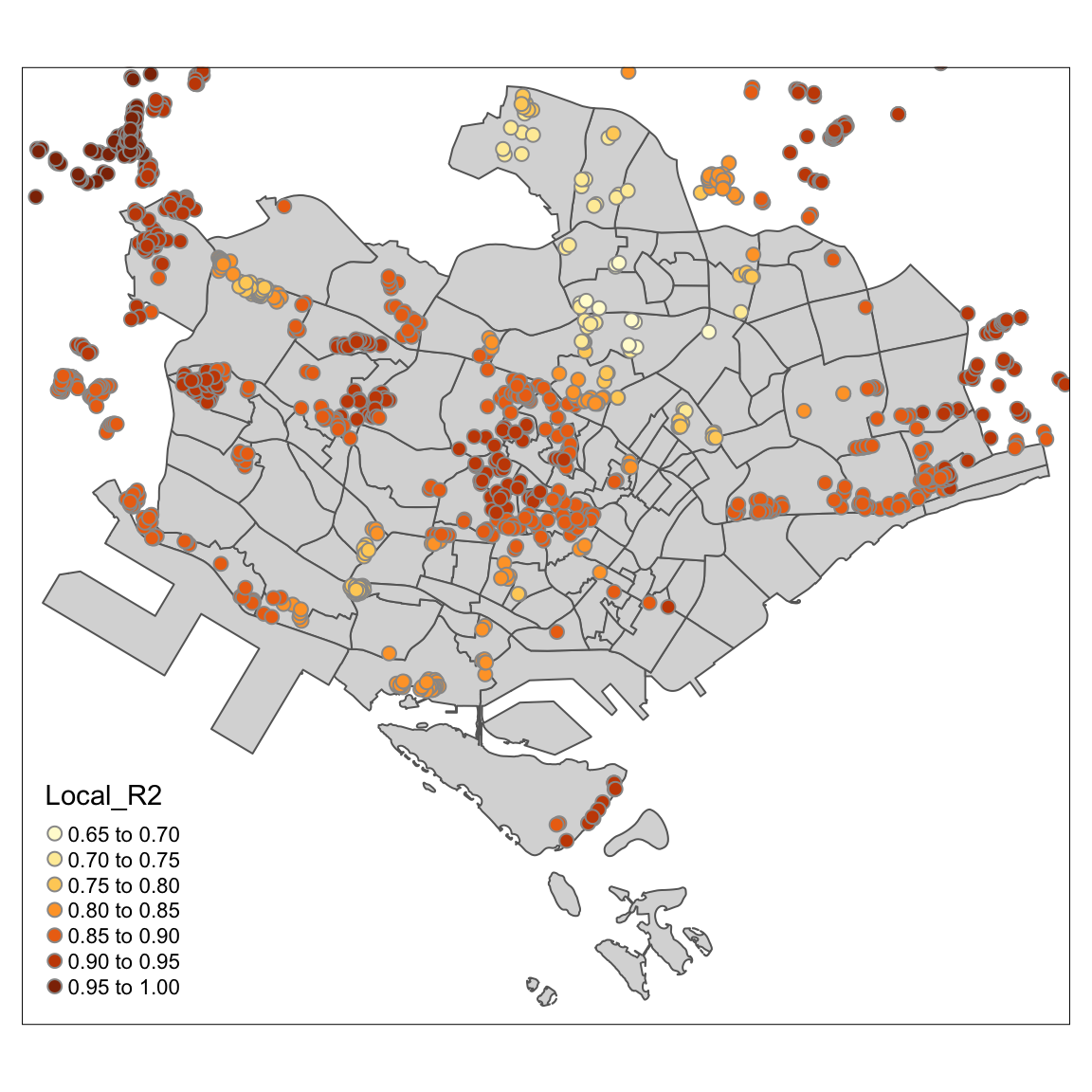
171347 1102001 1385528 1751842 1982307 13887901 10.5 Visualizing Local R2
The following code creates an interactive map showing local R2 values:
tmap_mode("view")
tm_shape(mpsz_svy21) +
tm_polygons(alpha = 0.1) +
tm_shape(condo_resale.sf.adaptive) +
tm_dots(col = "Local_R2", border.col = "gray60", border.lwd = 1) +
tm_view(set.zoom.limits = c(11, 14))tmap_mode("plot")10.6 Visualizing Coefficient Estimates
We can visualize the standard errors and t-values of the
AREA_SQM coefficient using the code below:
tmap_mode("view")
AREA_SQM_SE <- tm_shape(mpsz_svy21) +
tm_polygons(alpha = 0.1) +
tm_shape(condo_resale.sf.adaptive) +
tm_dots(col = "AREA_SQM_SE", border.col = "gray60", border.lwd = 1) +
tm_view(set.zoom.limits = c(11, 14))
AREA_SQM_TV <- tm_shape(mpsz_svy21) +
tm_polygons(alpha = 0.1) +
tm_shape(condo_resale.sf.adaptive) +
tm_dots(col = "AREA_SQM_TV", border.col = "gray60", border.lwd = 1) +
tm_view(set.zoom.limits = c(11, 14))
tmap_arrange(AREA_SQM_SE, AREA_SQM_TV, asp = 1, ncol = 2, sync = TRUE)tmap_mode("plot")10.6.1 By URA Planning Region
tm_shape(mpsz_svy21[mpsz_svy21$REGION_N == "CENTRAL REGION", ]) +
tm_polygons() +
tm_shape(condo_resale.sf.adaptive) +
tm_bubbles(col = "Local_R2", size = 0.15, border.col = "gray60", border.lwd = 1)