pacman::p_load(tidyverse, sf, tmap, ggstatsplot)In-Class Exercise 1
In the exercise, we will learn to handle geospatial data in R, create various maps, and perform statistical analysis using sf, tmap, and ggstatsplot.
1 Exercise Reference
2 Learning Outcome
-
Import and transform geospatial data using
tidyverseandsfpackages. - Analyze spatial datasets and extract meaningful insights.
-
Create and customize choropleth maps using the
tmappackage. - Develop analytical maps to visualize spatial patterns and distributions.
-
Perform statistical analysis on spatial data using the
ggstatsplotpackage. - Manage geospatial data workflows effectively in R.
3 Import the R Packages
| Package | Purpose | Use Case in Exercise |
|---|---|---|
| sf | Importing, managing, and processing geospatial data. | Handling and processing geospatial data in R. |
| tidyverse | Comprehensive set of tools for data science tasks. | Importing, wrangling, and visualizing data. |
| tmap | Creating thematic maps for visualizing spatial data. | Designing and displaying thematic maps to represent spatial patterns. |
| ggstatsplot | Enhancing ggplot2 plots with statistical analyses. | Adding statistical summaries and tests to visualizations for better insights. |
4 The Data
| Dataset | Source | Description |
|---|---|---|
| Master Plan 2014 Subzone Boundary (Web) | data.gov.sg | Geospatial boundaries for Singapore’s planning subzones in 2014. |
| Master Plan 2019 Subzone Boundary (Web) | data.gov.sg | Updated geospatial boundaries for Singapore’s planning subzones in 2019. |
| Pre-Schools Location | data.gov.sg | Location data for pre-schools in Singapore. |
| Singapore Residents by Planning Area / Subzone, Age Group, Sex and Type of Dwelling, June 2023 | singstat.gov.sg | Aspatial data on residents of Singapore by planning area, subzone, age, sex, and type of dwelling for June 2023. |
5 Working with Master Plan Planning Sub-zone Data
To import the shapefile version of the Sub-zone data:
mpsz14_shp <- st_read(dsn = "data",
                  layer = "MP14_SUBZONE_WEB_PL")
Reading layer `MP14_SUBZONE_WEB_PL' from data source
`/Users/walter/code/isss626/isss626-gaa/In-class_Ex/In-class_Ex01/data'
using driver `ESRI Shapefile'
Simple feature collection with 323 features and 15 fields
Geometry type: MULTIPOLYGON
Dimension: XY
Bounding box: xmin: 2667.538 ymin: 15748.72 xmax: 56396.44 ymax: 50256.33
Projected CRS: SVY21
Notice that mpsz14_shp is of class sf and
inherits from data.frame. This means it combines
spatial features with tabular data structure.
class(mpsz14_shp)[1] "sf" "data.frame"To import the kml version of the Sub-zone data:
mpsz14_kml <- st_read("data/MasterPlan2014SubzoneBoundaryWebKML.kml")
Note that this is a corrupted file. It is likely that the agency
has unknowingly uploaded a corrupted kml file.
To render a workable kml, we can convert the shp object and save it as a kml file.
st_write(mpsz14_shp,
         "data/MasterPlan2014SubzoneBoundaryWebKML.kml",
         delete_dsn=TRUE)
Note that the delete_dsn=TRUE argument ensures that any
existing file with the same name is deleted before saving the new
KML file, preventing potential conflicts or errors from overwriting.
To import pre-school location data in kml format:
preschool_kml <- st_read("data/PreSchoolsLocation.kml")Reading layer `PRESCHOOLS_LOCATION' from data source
`/Users/walter/code/isss626/isss626-gaa/In-class_Ex/In-class_Ex01/data/PreSchoolsLocation.kml'
using driver `KML'
Simple feature collection with 2290 features and 2 fields
Geometry type: POINT
Dimension: XYZ
Bounding box: xmin: 103.6878 ymin: 1.247759 xmax: 103.9897 ymax: 1.462134
z_range: zmin: 0 zmax: 0
Geodetic CRS: WGS 84To import Master Plan 2019 Subzone Boundary (No SEA) kml and MPSZ-2019 into sf simple feature data.frame:
mpsz19_shp <- st_read(dsn = "data",
                  layer = "MPSZ-2019") %>%
  st_transform(crs=3414)
Reading layer `MPSZ-2019' from data source
`/Users/walter/code/isss626/isss626-gaa/In-class_Ex/In-class_Ex01/data'
using driver `ESRI Shapefile'
Simple feature collection with 332 features and 6 fields
Geometry type: MULTIPOLYGON
Dimension: XY
Bounding box: xmin: 103.6057 ymin: 1.158699 xmax: 104.0885 ymax: 1.470775
Geodetic CRS: WGS 84mpsz19_kml <- st_read("data/MasterPlan2019RegionBoundaryNoSeaKML.kml")Reading layer `URA_MP19_REGION_NO_SEA_PL' from data source
`/Users/walter/code/isss626/isss626-gaa/In-class_Ex/In-class_Ex01/data/MasterPlan2019RegionBoundaryNoSeaKML.kml'
using driver `KML'
Simple feature collection with 5 features and 2 fields
Geometry type: MULTIPOLYGON
Dimension: XYZ
Bounding box: xmin: 103.6057 ymin: 1.158699 xmax: 104.0885 ymax: 1.470775
z_range: zmin: 0 zmax: 0
Geodetic CRS: WGS 846 Handling Coordinate Systems
To check the project of the imported sf objects:
st_crs(mpsz19_shp)Coordinate Reference System:
User input: EPSG:3414
wkt:
PROJCRS["SVY21 / Singapore TM",
BASEGEOGCRS["SVY21",
DATUM["SVY21",
ELLIPSOID["WGS 84",6378137,298.257223563,
LENGTHUNIT["metre",1]]],
PRIMEM["Greenwich",0,
ANGLEUNIT["degree",0.0174532925199433]],
ID["EPSG",4757]],
CONVERSION["Singapore Transverse Mercator",
METHOD["Transverse Mercator",
ID["EPSG",9807]],
PARAMETER["Latitude of natural origin",1.36666666666667,
ANGLEUNIT["degree",0.0174532925199433],
ID["EPSG",8801]],
PARAMETER["Longitude of natural origin",103.833333333333,
ANGLEUNIT["degree",0.0174532925199433],
ID["EPSG",8802]],
PARAMETER["Scale factor at natural origin",1,
SCALEUNIT["unity",1],
ID["EPSG",8805]],
PARAMETER["False easting",28001.642,
LENGTHUNIT["metre",1],
ID["EPSG",8806]],
PARAMETER["False northing",38744.572,
LENGTHUNIT["metre",1],
ID["EPSG",8807]]],
CS[Cartesian,2],
AXIS["northing (N)",north,
ORDER[1],
LENGTHUNIT["metre",1]],
AXIS["easting (E)",east,
ORDER[2],
LENGTHUNIT["metre",1]],
USAGE[
SCOPE["Cadastre, engineering survey, topographic mapping."],
AREA["Singapore - onshore and offshore."],
BBOX[1.13,103.59,1.47,104.07]],
ID["EPSG",3414]]Next, re-write the code chunk to import the Master Plan Sub-zone 2019 and Pre-schools Location with proper transformation.
mpsz19_shp <- st_read(dsn = "data/",
                layer = "MPSZ-2019") %>%
  st_transform(crs = 3414)
Reading layer `MPSZ-2019' from data source
`/Users/walter/code/isss626/isss626-gaa/In-class_Ex/In-class_Ex01/data'
using driver `ESRI Shapefile'
Simple feature collection with 332 features and 6 fields
Geometry type: MULTIPOLYGON
Dimension: XY
Bounding box: xmin: 103.6057 ymin: 1.158699 xmax: 104.0885 ymax: 1.470775
Geodetic CRS: WGS 84preschool <- st_read("data/PreSchoolsLocation.kml") %>%
st_transform(crs = 3414)Reading layer `PRESCHOOLS_LOCATION' from data source
`/Users/walter/code/isss626/isss626-gaa/In-class_Ex/In-class_Ex01/data/PreSchoolsLocation.kml'
using driver `KML'
Simple feature collection with 2290 features and 2 fields
Geometry type: POINT
Dimension: XYZ
Bounding box: xmin: 103.6878 ymin: 1.247759 xmax: 103.9897 ymax: 1.462134
z_range: zmin: 0 zmax: 0
Geodetic CRS: WGS 847 Geospatial Data Wrangling
7.1 Point-in-Polygon count
The code below counts the number of preschools within each
planning subzone. It uses st_intersects to find
intersections between the geometries of the subzones
(mpsz19_shp) and the preschool locations, identifying
where the two sets of geometries overlap or share common points.
The
lengths()
function is then applied to count the number of intersecting
preschools for each subzone, effectively returning the total
number of preschools within each subzone in the
mpsz19_shp shapefile.
mpsz19_shp <- mpsz19_shp %>%
  mutate(`PreSch Count` = lengths(
    st_intersects(mpsz19_shp, preschool)))
7.2 Computing Density
The code below performs the following tasks:
Derive the area of each planning sub-zone.
Drop the unit of measurement of the area (i.e. m^2)
Calculate the density of pre-school at the planning sub-zone level.
mpsz19_shp <- mpsz19_shp %>%
  mutate(Area = units::drop_units(
    st_area(.)),
    `PreSch Density` = `PreSch Count` / Area * 1000000
  )
8 Statistical Analysis
In this section, we will use appropriate Exploratory Data Analysis (EDA) and Confirmatory Data Analysis (CDA) methods to explore and confirm the statistical relationship between Pre-school Density and Pre-school count.
# Convert the 'PreSch Density' column in 'mpsz19_shp' to numeric format
mpsz19_shp$`PreSch Density` <- as.numeric(as.character(mpsz19_shp$`PreSch Density`))
# Convert the 'PreSch Count' column in 'mpsz19_shp' to numeric format
mpsz19_shp$`PreSch Count` <- as.numeric(as.character(mpsz19_shp$`PreSch Count`))
# Convert the spatial data frame 'mpsz19_shp' to a regular data frame for plotting
mpsz19_df <- as.data.frame(mpsz19_shp)
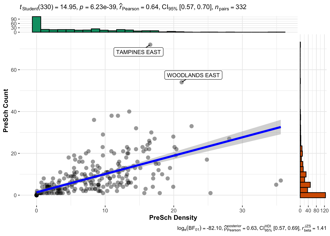
# Create a scatter plot with statistical details using the 'ggscatterstats' function from the 'ggstatsplot' package
ggstatsplot::ggscatterstats(data = mpsz19_df,
x = `PreSch Density`, # Set 'PreSch Density' as the x-axis variable
y = `PreSch Count`, # Set 'PreSch Count' as the y-axis variable
type = "parametric", # Specify the type of statistical test to use (parametric)
label.var = SUBZONE_N, # Label points with the subzone names
label.expression = `PreSch Count` > 40) # Label only those points where 'PreSch Count' is greater than 40
Note
Output Intepretation:
The plot shows a moderately strong positive correlation between preschool density and the number of preschools in each subzone. As the preschool density increases, the number of preschools tends to increase as well.
9 Working with Population data
popdata <- read_csv("data/respopagesextod2023.csv")To prepare a data.frame showing population by Planning Area and Planning subzone:
popdata2023 <- popdata %>%
  # Group the data by Planning Area (PA), Subzone (SZ), and Age Group (AG)
  group_by(PA, SZ, AG) %>%
  # Summarize the population (POP) by calculating the sum of 'Pop' within each group
  summarise(`POP` = sum(`Pop`)) %>%
  # Remove the grouping structure to avoid issues in further operations
  ungroup() %>%
  # Reshape the data to a wider format: create separate columns for each Age Group (AG)
  # with their corresponding population values (POP)
  pivot_wider(names_from = AG, values_from = POP)

colnames(popdata2023)
[1] "PA" "SZ" "0_to_4" "10_to_14" "15_to_19"
[6] "20_to_24" "25_to_29" "30_to_34" "35_to_39" "40_to_44"
[11] "45_to_49" "50_to_54" "55_to_59" "5_to_9" "60_to_64"
[16] "65_to_69" "70_to_74" "75_to_79" "80_to_84" "85_to_89"
[21] "90_and_Over"Now, we will perform data processing to derive a tibble data.framewith the following fields PA, SZ, YOUNG, ECONOMY ACTIVE, AGED, TOTAL, DEPENDENCY where by:
- YOUNG: age group 0 to 4 until age groyup 20 to 24,
- ECONOMY ACTIVE: age group 25-29 until age group 60-64,
- AGED: age group 65 and above,
- TOTAL: all age group, and
- DEPENDENCY: the ratio between young and aged against economy active group.
popdata2023 <- popdata2023 %>%
  # Calculate the 'YOUNG' population: sum of age groups 0-24, 10-24, and 5-9
  mutate(YOUNG = rowSums(.[3:6]) + rowSums(.[14])) %>%
  # Calculate the 'ECONOMY ACTIVE' population: sum of age groups 25-59 and 60-64
  mutate(`ECONOMY ACTIVE` = rowSums(.[7:13]) + rowSums(.[15])) %>%
  # Calculate the 'AGED' population: sum of age groups 65 and above
  mutate(`AGED` = rowSums(.[16:21])) %>%
  # Calculate the 'TOTAL' population: sum of all age groups
  mutate(`TOTAL` = rowSums(.[3:21])) %>%
  # Calculate the 'DEPENDENCY' ratio: (YOUNG + AGED) / ECONOMY ACTIVE
  mutate(`DEPENDENCY` = (`YOUNG` + `AGED`) / `ECONOMY ACTIVE`) %>%
  # Select only the relevant columns to keep in the final data frame
  select(`PA`, `SZ`, `YOUNG`, `ECONOMY ACTIVE`, `AGED`, `TOTAL`, `DEPENDENCY`)
Next, we will joining aspatial and geospatial data. First, we use
toupper()
to convert elements of PA and SZ to upper case.
popdata2023 <- popdata2023 %>%
  mutate_at(.vars = vars(PA, SZ),
          .funs = list(toupper))
The code below demonstrates how to use left_join() to
merge the geospatial data mpsz19_shp with the
population data popdata2023. By keeping
mpsz19_shp as the left table in the first join, we
ensure that the geometry details of the spatial data are preserved:
mpsz_pop2023 <- left_join(mpsz19_shp, popdata2023,
                          by = c("SUBZONE_N" = "SZ"))
In contrast, the second join keeps popdata2023 as the
left table, meaning the population data is retained, and geometry
details from mpsz19_shp are added where they match:
pop2023_mpsz <- left_join(popdata2023, mpsz19_shp,
                          by = c("SZ" = "SUBZONE_N"))
10 Choropleth Map of Dependency Ratio by Planning Subzone
# Set the base shape for the map using the merged geospatial and population data
tm_shape(mpsz_pop2023) +

  # Fill the map areas based on the "DEPENDENCY" variable, using a quantile classification and a blue color palette
  tm_fill("DEPENDENCY",
          style = "quantile",
          palette = "Blues",
          title = "Dependency ratio") +

  # Customize the layout of the map with a title and legend adjustments
  tm_layout(main.title = "Distribution of Dependency Ratio by planning subzone",
            main.title.position = "center",
            main.title.size = 1,
            legend.title.size = 1,
            legend.height = 0.45,
            legend.width = 0.35) + # Corrected: add "+" to continue chaining elements

  # Add semi-transparent borders around the subzones
  tm_borders(alpha = 0.5) +

  # Add compass with a star-shaped style
  tm_compass(type = "8star", size = 1.5) +

  # Add scale bar
  tm_scale_bar() +

  # Add grid to map
  tm_grid(alpha = 0.2) +

  # Cite the data source
  tm_credits("Source: Planning Sub-zone boundary from Urban Redevelopment Authority (URA)\n and Population data from Department of Statistics (DOS)",
             position = c("left", "bottom"))

Note
The output is a choropleth map showing the distribution of the dependency ratio by planning subzone in Singapore.
-
The map clearly shows which areas have higher or lower dependency ratios. For instance, darker areas like certain central regions have higher dependency ratios, suggesting a higher number of dependents (both young and aged) compared to the working-age population.
-
Lighter areas have lower ratios, indicating a balance or a larger working-age population compared to dependents.
11 Analytical Map: Percentile Map
The percentile map is a special type of quantile map with six specific categories: 0-1%,1-10%, 10-50%,50-90%,90-99%, and 99-100%. The corresponding breakpoints can be derived by means of the base R quantile command, passing an explicit vector of cumulative probabilities as c(0,.01,.1,.5,.9,.99,1). Note that the begin and endpoint need to be included.
First, we have to process the data by dropping NA records.
mpsz_pop2023 <- mpsz_pop2023 %>%
  drop_na()
Next, we defines a function to get the input data and field to be used for creating the percentile map.
Then, we creates a percentile mapping function for computing and plotting the percentile map.
# Create a percentile map based on a variable
percentmap <- function(vnam, df, legtitle = NA, mtitle = "Percentile Map") {
  # Define percentile breaks to be used for map legend
  percent <- c(0, .01, .1, .5, .9, .99, 1)

  # Retrieve the variable from the data frame based on the variable name
  var <- get.var(vnam, df)

  # Calculate the percentile values (break points) for the variable
  bperc <- quantile(var, percent)

  # Create the base shape layer using the mpsz_pop2023 dataset
  tm_shape(mpsz_pop2023) +
  tm_polygons() + # Draw polygons for subzones

  # Overlay the specified data frame 'df' on the map
  tm_shape(df) +
     tm_fill(vnam, # Fill polygons based on the variable 'vnam'
             title = legtitle, # Set legend title
             breaks = bperc, # Use calculated percentiles for breaks
             palette = "Blues", # Apply a blue color palette
             labels = c("< 1%", "1% - 10%", "10% - 50%", "50% - 90%", "90% - 99%", "> 99%"))  +
  tm_borders() + # Add borders to the map polygons

  # Customize the layout and appearance of the map
  tm_layout(main.title = mtitle, # Set the main title of the map
            title.position = c("right", "bottom"))
}
Finally, we can plot the percentile map.
percentmap("DEPENDENCY", mpsz_pop2023)

12 Analytical Map: Box Map
In essence, a box map is an augmented quartile map, with an additional lower and upper category. When there are lower outliers, then the starting point for the breaks is the minimum value, and the second break is the lower fence. In contrast, when there are no lower outliers, then the starting point for the breaks will be the lower fence, and the second break is the minimum value (there will be no observations that fall in the interval between the lower fence and the minimum value).
- Create the
boxbreaksfunction
The code block below is an R function that creating break points for a box map.
-
arguments:
- v: vector with observations
- mult: multiplier for IQR (default 1.5)
-
returns:
- bb: vector with 7 break points compute quartile and fences
# int a function 'boxbreaks' to calculate break points based on boxplot statistics
boxbreaks <- function(v, mult = 1.5) {
  # Calculate the quartiles of the input vector 'v' and remove names
  qv <- unname(quantile(v))

  # Calculate the interquartile range (IQR)
  iqr <- qv[4] - qv[2]

  # Calculate the upper and lower fences for outlier detection
  upfence <- qv[4] + mult * iqr
  lofence <- qv[2] - mult * iqr

  # Initialize a numeric vector 'bb' with 7 elements to store the break points
  bb <- vector(mode = "numeric", length = 7)

  # Determine lower break points based on lower fence
  if (lofence < qv[1]) {  # No lower outliers
    bb[1] <- lofence      # Set lower fence as the first break point
    bb[2] <- floor(qv[1]) # Round down to the nearest integer for the next break point
  } else {                # There are lower outliers
    bb[2] <- lofence      # Set lower fence as the second break point
    bb[1] <- qv[1]        # Set the minimum value as the first break point
  }

  # Determine upper break points based on upper fence
  if (upfence > qv[5]) {  # No upper outliers
    bb[7] <- upfence      # Set upper fence as the last break point
    bb[6] <- ceiling(qv[5]) # Round up to the nearest integer for the previous break point
  } else {                # There are upper outliers
    bb[6] <- upfence      # Set upper fence as the sixth break point
    bb[7] <- qv[5]        # Set the maximum value as the last break point
  }

  # Set the inner quartile values (Q1, Median, Q3) as middle break points
  bb[3:5] <- qv[2:4]

  return(bb)
}- Create the
get.varfunction
The R function below extracts a variable as a vector out of an sf data frame.
-
arguments:
- vname: variable name (as character, in quotes)
- df: name of sf data frame
-
returns:
- v: vector with values (without a column name)
# init  a function 'get.var' to extract a variable from a data frame without its spatial geometry
get.var <- function(vname, df) {
  # Select the specified variable 'vname' from the data frame 'df' and remove the spatial geometry information
  v <- df[vname] %>%
    st_set_geometry(NULL) # Remove the geometry component from the sf object to get a plain data frame

  # Remove the column name from the variable and convert it to a plain vector
  v <- unname(v[,1])

  return(v)
}- Create the Boxmap function
The code chunk below is an R function to create a box map.
-
arguments:
- vnam: variable name (as character, in quotes)
- df: simple features polygon layer
- legtitle: legend title
- mtitle: map title
- mult: multiplier for IQR
-
returns:
- a tmap-element (plots a map)
# Define a function 'boxmap' to create a box map based on a variable
boxmap <- function(vnam, df,
                   legtitle = NA, # Set default value for legend title as NA
                   mtitle = "Box Map", # Set default value for main title
                   mult = 1.5) { # Set default multiplier for calculating fences in boxplot

  # Extract the variable data from the data frame without geometry
  var <- get.var(vnam, df)

  # Calculate the break points for the box map using the 'boxbreaks' function
  bb <- boxbreaks(var)

  # Create the base shape layer using the specified data frame 'df'
  tm_shape(df) +
    tm_polygons() + # Draw polygons for spatial units

  # Overlay the data frame again to apply fill color based on the variable
  tm_shape(df) +
     tm_fill(vnam, # Fill polygons based on the variable 'vnam'
             title = legtitle, # Set legend title
             breaks = bb, # Use calculated boxplot breaks for coloring
             palette = "Blues", # Apply a blue color palette
             labels = c("Lower outlier",  # Label for lower outliers
                        "< 25%",          # Label for first quartile
                        "25% - 50%",      # Label for second quartile (median)
                        "50% - 75%",      # Label for third quartile
                        "> 75%",          # Label for upper quartile
                        "Upper outlier")) + # Label for upper outliers
  tm_borders() + # Add borders to the polygons on the map

  # Customize the layout and appearance of the map
  tm_layout(main.title = mtitle, # Set the main title of the map
            title.position = c("left", "top"), # Position the title at the top left
            frame = F) # Remove the map frame
}- Finally, plot the Box Map
Static Box Map
boxmap("DEPENDENCY", mpsz_pop2023)

Interactive Box Map
tmap_options(check.and.fix = TRUE)
tmap_mode("view")
tm_basemap("Esri.WorldGrayCanvas") +
boxmap("DEPENDENCY", mpsz_pop2023)